Báo cáo hóa học: " Algorithms for Blind Components Separation and Extraction from the Time-Frequency Distribution of Their Mixture" docx
Bạn đang xem bản rút gọn của tài liệu. Xem và tải ngay bản đầy đủ của tài liệu tại đây (1.31 MB, 9 trang )
EURASIP Journal on Applied Signal Processing 2004:13, 2025–2033
c
2004 Hindawi Publishing Corporation
Algorithms for Blind Components Separation
and Extraction from the Time-Frequency
Distribution of Their Mixture
B. Barkat
School of Electrical and Electronic Enginee ring, Nanyang Technological University, Nanyang Avenue, 639798 Singapore
Email:
K. Abed-Meraim
Signal and Image Processing Department,
´
Ecole National Sup
´
erieure des T
´
el
´
ecommunications, Telecom Paris, 75013 Paris, France
Email:
Received 20 February 2003; Revised 29 November 2003; Recommended for Publication by Petar Djuri
´
c
We propose novel algorithms to select and extract separately all the components, using the time-frequency distribution (TFD),
of a given multicomponent frequency-modulated (FM) signal. These algorithms do not use any a priori information about the
various components. However, their performances highly depend on the cross-terms suppression ability and high time-frequency
resolution of the considered TFD. To illustrate the usefulness of the proposed algorithms, we applied them for the estimation of the
instantaneous frequency coefficients of a multicomponent signal and the results are compared with those of the higher-order am-
biguity function (HAF) algorithm. Monte Carlo simulation results show the superiority of the proposed algorithms over the HAF.
Keywords and phrases: time-frequency signal analysis, components separation, polynomial phase signals, instantaneous fre-
quency estimation.
1. INTRODUCTION
Thejointtime-frequencyanalysishasprovedtobeapower-
ful tool in the analysis of nonstationary signals, that is, sig-
nals whose spectral contents vary with time [1]. Such sig-
nals may be found in many engineering applications such as
radar, sonar, telecommunications, and biomedical engineer-
ing. These signals can be classified in two groups: monocom-
ponent and multicomponent.
In this paper, we focus our analysis on multicomponent
signals. By a multicomponent signal, we mean a signal w hose
time-frequency representation presents multiple ridges in
the time-frequency plane. Analytically, it may be defined as
s(t) =
M
i=1
s
i
(t), (1)
where each component s
i
(t), of the form
s
i
(t) = a
i
(t)e
jφ
i
(t)
,(2)
is assumed to have only one ridge, or one continuous curve,
in the time-frequency plane. An example of a multicompo-
nent signal, consisting of three components, is displayed in
Figure 1.
Recovery of a particular component from a given multi-
component signal has always been a challenge for the time-
frequency community. The objective of this paper is to ad-
dress this particular problem. Specifically, we present two dif-
ferent algorithms in order to retrieve and extract separately
the components from the time-frequency distribution (TFD)
of their mixture signal. The motivation behind this can be
found in situations where the user may be interested in the
instantaneous frequency ( IF) law of one of the components
only. For instance, in telecommunications the received signal
may be a mixture of several source signals (multiple access in-
terference) but the user may wish to recover only one source
signal (blind source separation) [2, 3]. In this context, by ap-
plying either of the proposed algorithms to the TFD of the
received signal, we may be able to separate and recover the
desired source signal.
The algorithms proposed here do not use any a priori
information about the various components to be extracted.
However, the first algorithm assumes that all components
of the signal exist at the almost all time instants; while, the
second algorithm assumes that all components are well sep-
arated in the time-frequency plane. Moreover, it is necessary
that the used TFD, in addition to its high time-frequency
2026 EURASIP Journal on Applied Signal Processing
0.450.40.350.30.250.20.150.10.05
Frequency (Hz)
50
100
150
200
250
300
350
400
450
500
Time (s)
Figure 1: A t ime-frequency distribution of a multicomponent sig-
nal. F
s
= 1Hz,N = 512, Time resolution = 1.
resolution, should be cross-terms free or at least be able to
suppress them as much as possible.
Once the various components have been extracted, we
can use available estimation techniques to obtain their de-
sired char acteristics [4]. In the literature, we can find other
techniques for the estimation of multicomponent signals in
noise [5, 6, 7]. Among these we can cite the higher-order
ambiguity function (HAF) algorithm [7]. Explicitly, the al-
gorithm in [7] was designed to estimate the phase parame-
ters as well as the constant, or slowly varying, amplitudes of
each component of a multicomponent signal. Each of these
components is assumed to have a polynomial phase law. As
an illustration, we present here a brief statistical performance
comparison between one of the proposed algorithms and the
HAF in the estimation of a multicomponent signal consist-
ing of two quadratic polynomial phase signals embedded in
noise. We note that our proposed algorithms can also be used
in the estimation of other nonlinear, not necessarily polyno-
mial, phase signals. Examples, using real-life as well as syn-
thetic data, are presented in order to show the high accuracy
of the proposed algorithms.
The paper is organized as follows. In Section 2, we dis-
cuss the choice of the appropriate TFD to be used in both
algorithms. In Section 3, we present the first algorithm as
well as the statistical comparison with the HAF algorithm. In
Section 4, we present the second algorithm. Section 5 con-
cludes the paper.
2. TIME-FREQUENCY DISTRIBUTION CHOICE
There exist many TFDs. The choice of a TFD depends on the
specific application at hand and the representation properties
that are desirable for this application. One of the well-known
TFDs is the Wigner-Ville distribution (WVD) defined as [1]
W(t, f ) =
+∞
−∞
z
t +
τ
2
· z
∗
t −
τ
2
e
− j2πfτ
dτ,(3)
where z(t) is the analytic version of the signal under consid-
eration.
0.450.40.350.30.250.20.150.10.05
Frequency (Hz)
50
100
150
200
250
300
350
400
450
500
Time (s)
Figure 2: The WVD of the same multicomponent signal displayed
in Figure 1. F
s
= 1Hz,N = 512, Time resolution = 1.
The WVD is known to have high resolution in both time
and frequency; however, it suffers from the presence of cross-
terms for a multicomponent signal. These cross-terms result
from the interaction of different components of the signal. As
an illustration, we consider the WVD of the multicomponent
signal displayed in Figure 1. The WVD of such a signal is dis-
played in Figure 2. It is clear from this figure that the features
of the signal are hidden making the WVD inappropriate for
the analysis in this case.
In order to apply the proposed algorithms we need to
have a “clean” TFD. That is, we need a distribution that can
reveal the features of the signal as clearly as possible without
any “ghost” component. For that, we need to apply a TFD
that can get rid of the cross-terms while preserving a h igh
time-frequency resolution. Thanks to the recent results in the
design of TFDs, nowadays the user has a myriad of TFDs to
choose from [8, 9, 10, 11]. As an example, in the sequel, we
will use a newly developed high-resolution quadratic TFD.
This distribution, called the B-distribution, is defined as [12]
S(t, f )=
+∞
−∞
|τ|
cosh(t
)
σ
·
z
t − t
+
τ
2
· z
∗
t − t
−
τ
2
· e
− j2πfτ
dt
dτ,
(4)
where 0 ≤ σ ≤ 1 is a real parameter. The choice of the B-
distribution, or its modified version [13], stems from the fact
that it presents a good performance in terms of resolution
and cross-terms suppression. Detailed performance evalua-
tion, design criteria, and implementation can be found in
[12, 13]. In Figure 1, it was this particular distribution that
was used to display the time-frequency representation of the
signal.
In the next sections, we will present the two proposed
algorithms to select and extract a particular component (of
a given multicomponent signal) using the B-distribution.
However, we should s tress here that any other clean, with
high resolution, TFD can also be used. For instance, in [14]
we used the S-distribution [10] to successfully extract the
various components of the multicomponent signal.
Blind Components Separation and Extraction Using TFD 2027
Masking
Masking
Masking
.
.
.
.
.
.
Cd(t, f )
Ci(t, f )
C1( t, f )
C1
Ci
Cd
Components
separation
(Algorithm 2)
d
T
th
(t, f )
Input 1D
signal
s(t)
Signal TFD
(B-distribution)
T(t, f )
Noise
thresholding
Estimation
of the number
of components
Figure 3: Flowchart of the proposed first algorithm.
3. PROPOSED FIRST ALGORITHM
The first proposed components-separation algorithm is il-
lustrated in Figure 3, and Algorithms 1 and 2. Figure 3 pro-
vides the algorithm flowchart, Algorithm 1 summarizes the
estimation technique of the number of components, and
Algorithm 2 summarizes the components-separation tech-
nique.
The first step of the algorithm consists in noise thresh-
olding to remove the undesired “low” energy peaks in the
time-frequency domain
1
.Thisoperationcanbewrittenas
T
th
(t, f ) =
T(t, f )ifT(t, f ) > ,
0 otherwise,
(5)
where
is a properly chosen threshold (in our simulations
we used = 0.01 max
(t, f )
T(t, f )).
The second step consists in estimating the number of
components as shown next.
3.1. Estimation of the number of components
First, we assume that all components exist simultaneously at
almost all time instants in the time-frequency plane. Second,
we observe that, in general, for a noiseless and cross-terms
free TFD, the number of components at a given time instant
t
0
can be estimated as the number of peaks of the TFD slice
T(t
0
, f ). By searching and counting the peaks of each TFD
slice, we end up w ith a set of numbers. The number corre-
sponding to the maximum of the histogram of these num-
bers yields an estimate of the number of components in the
signal. This simple procedure is detailed in Algorithm 1.
Note that the thresholding operation performed in the
first step has an effect on the second step. Indeed, the TFD
should present high peaks for the auto-terms compared to
cross-terms and noise. In this situation, the threshold can
easily remove all peaks that do not belong to auto-terms.
1
This noise thresholding is justified by the fact that the noise energy i s
spread over all time-frequency domain while the components energies are
well localized around their respective IFs leading to high energy peaks for
the latter (assuming no cross-terms).
(1) For each time instant t,wheret = 1, , t
max
, take a slice
of the TFD T(t, f ).
(2) Search and count the number of peaks in each slice.
(3) Evaluate the histogram of the obtained set of peaks
numbers.
(4) Estimate the total number of the signal components as
the argument of the maximum of the above histogram.
Algorithm 1: Estimation of the number of components.
(1) Assign an index to each of the d components in an
orderly manner.
(2) For each time instant t (starting from t = 1) find the
components frequencies as the peaks positions of the
TFD slice T(t, f ).
(3) Assig n a peak to a particular component based on the
smallest distance to the peaks of the previous slice
T(t − 1, f )(IFscontinuousfunctionsoftime).Forthe
special case of a crossing point (see step (4) how to
detect it and its corresponding components), we assign
the peak to both crossing components.
(4) If at a time instant t a crossing point exists (i.e., number
of peaks smaller than the number of components), iden-
tify the crossing components using the smallest distance
criterion by comparing the distances of the actual peaks
to those of the previous slice.
(5) Permute the indices of the corresponding crossing
components.
Algorithm 2: Components-separation procedure for the proposed
first algorithm.
However, in large noise situations the choice of the threshold
value becomes more difficult and this may generate errors in
the number of components.
3.2. Components-separation procedure
The proposed algorithm assumes that (i) all components ex-
ist at all time instants in the time-frequency plane and (ii) any
components intersection is a crossing point. Under these two
assumptions, we note that if, at a time instant t
0
,twocompo-
nents are crossing, then the number of peaks ( at this partic-
ular slice T(t
0
, f )) is smaller than the total number of com-
ponents d. For practical implementation reasons, we decide
that a crossing occurs when the number of peaks is smaller
than d over a fixed number of consecutive slices. In this case,
we implement the following procedure:
(1) choose a particular maximum point location in the
slice where the crossing occurs;
(2) measure all distances from this point to the peaks lo-
cations of the previous slice (with no crossing);
(3) select the 2 smallest distances and add them;
(4) repeat steps (1) to (3) for a ll other maximum point
locations in the slice where the crossing occurred;
2028 EURASIP Journal on Applied Signal Processing
0.40.30.20.10
Frequency (Hz)
0
100
200
300
400
500
Time (s)
0.40.30.20.10
Frequency (Hz)
0
100
200
300
400
500
Time (s)
0.40.30.20.10
Frequency (Hz)
0
100
200
300
400
500
Time (s)
0.40.30.20.10
Frequency (Hz)
0
100
200
300
400
500
Time (s)
Figure 4: The B-distribution of the original signal (top left) as well as the extracted components using the proposed first algorithm.
(5) from the set of the smallest sums found above, the pro-
gram selects the smallest value and the points associ-
ated to them. This w ill yield the location where the
crossing occurred and the 2 components involved in
the crossing.
Then, we use a simple numerical permutation opera-
tion of the 2 components involved in the crossing. The de-
tails of the proposed separation technique is outlined in
Algorithm 2.
To validate the proposed algorithm, we reconsider the
same multicomponent signal analysed earlier. This signal
consists of a mixture of a unit modulus (with increasing fre-
quency) quadratic frequency-modulated (FM) component,
a unit modulus (with decreasing frequency) quadratic FM
component, and a unit modulus (with increasing frequency)
linear FM component. The mixture signal is added to a zero-
mean white Gaussian noise with power equal to 0 dB. This
means that the individual signal-to-noise r atio (SNR) de-
fined as SNR
i
= ith component power/noise power is equal
to 0 dB.
The B-distribution of the noisy signal as well as the com-
ponents resulting from the separation algorithm are dis-
played in Figure 4.
Adifferent signal consisting of 5 components was also
analysed using the proposed algorithm. In particular, this sig-
nal is a mixture of two linear FM signals, a quadratic FM
signal, a cubic FM signal, and a pure sinusoid. The mixture
signal was embedded in 0 dB Gaussian noise. Similarly to the
previous case, the individual SNR is also equal to 0 dB. Again,
the algorithm was able to separate and extract each of these
components. The results are displayed in Figure 5.
Note that a similar algorithm to the one above could be
designed if the signal exists over all frequencies but not nec-
essarily over all times. In this case, the slices are taken at par-
ticular frequencies and not time instants as we did here.
3.3. Performance evaluation and comparison
In this subsection, we evaluate the statistical performance of
the proposed first algorithm and compare it to the perfor-
mance of the HAF method [7]. For that, consider a discrete-
time multicomponent signal consisting of two linear FM
components embedded in additive white complex Gaussian
noise w(n):
y(n)
= z
1
+ z
2
+ w(n), n = 0, 1, , N − 1, (6)
where z
1
= exp{ j(a
1
n + a
2
n
2
)} and z
2
= exp{ j(b
1
n + b
2
n
2
)}.
The noise w(n) is assumed to be an independent and identi-
cally distributed (i.i.d.) sequence with zero mean and vari-
ance equal to σ
2
. The signals’ IF coefficients are given by
a
1
= 0.4π, a
2
= 0.5π10
−3
, b
1
= 0.9π,andb
2
=−1.5π10
−3
.
ThesignallengthischosenequaltoN = 256 with a sam-
pling per iod equal to unity. We define the SNR as the total
noiseless signal power over the noise power, namely,
SNR (dB) = 10log
10
z
1
2
+
z
2
2
σ
2
. (7)
For a given SNR value, we put the noisy signal y(n) through
the proposed algorithm in order to extract the two respective
components. The peaks of the extracted components (in the
time-frequency domain) are then used to estimate the IFs of
Blind Components Separation and Extraction Using TFD 2029
0.40.20
Frequency (Hz)
0
100
200
300
400
500
Time (s)
0.40.20
Frequency (Hz)
0
100
200
300
400
500
Time (s)
0.40.20
Frequency (Hz)
0
100
200
300
400
500
Time (s)
0.40.20
Frequency (Hz)
0
100
200
300
400
500
Time (s)
0.40.20
Frequency (Hz)
0
100
200
300
400
500
Time (s)
0.40.20
Frequency (Hz)
0
100
200
300
400
500
Time (s)
Figure 5: The B-distribution of a different multicomponent signal (top left) as well as the extracted components using the proposed first
algorithm.
these linear FM components [4]. By recalling that the IF of
z
1
(n) (estimated f rom the peak of the extracted component)
is given by [4]:
f
z
1
(n) =
1
2π
·
a
1
+2a
2
· n
, n = 0, , N − 1, (8)
and that of z
2
(n) (estimated from the peak of the other ex-
tracted component) is given by
f
z
2
(n) =
1
2π
·
b
1
+2b
2
· n
, n = 0, , N − 1, (9)
we use a simple polynomial fit to obtain estimates of (a
1
, a
2
)
from f
z
1
(n)andestimatesof(b
1
, b
2
)from f
z
2
(n).
For comparison purposes, the same noisy signal y(n)is
also put through the HAF algorithm [7]. From this algo-
rithm, we directly obtain the IF coefficients estimates [7].
These estimates are then used to evaluate the corresponding
IFs estimates of the two linear FM components (using the
above expressions). We note here that, in the comparison, we
choose the coefficients to be half of those of [7] to contain the
frequency in the range 0–0.5 Hz instead of the 0–1 Hz. More-
over, in the simulation, we used a second estimation stage as
suggested in [7] to refine the phase parameter estimates.
In Figure 6, we display the estimated IFs of the two
components. The dotted lines correspond to the HAF algo-
rithm and the dashed lines correspond to the proposed first
algorithm. The true IFs are represented by the continuous
300250200150100500
Time (s)
0.05
0.1
0.15
0.2
0.25
0.3
0.35
0.4
0.45
0.5
Instantaneous frequencies (Hz)
Tru e IFs
IFs estimated (new algorithm)
IFs estimated (HAF)
Figure 6: Estimated IFs of the two linear FM components. The dot-
ted lines correspond to the HAF algorithm and the dashed-dotted
lines correspond to the proposed first algorithm.
lines (superimposed with those of the proposed first algo-
rithm). The superiority of the proposed algorithm over the
HAF is obvious. In this particular example, the SNR was fixed
equal to 0 dB.
2030 EURASIP Journal on Applied Signal Processing
6420−2
SNR (dB)
−100
−90
−80
−70
−60
−50
−40
MSE (dB)
2-stage HAF algorithm
1-stage HAF algorithm
Proposed first algorithm
6420−2
SNR (dB)
−50
−40
−30
−20
−10
0
10
MSE (dB)
2-stage HAF algorithm
1-stage HAF algorithm
Proposed first algorithm
6420−2
SNR (dB)
−100
−90
−80
−70
−60
−50
−40
MSE (dB)
2-stage HAF algorithm
1-stage HAF algorithm
Proposed first algorithm
6420−2
SNR (dB)
−50
−40
−30
−20
−10
0
10
MSE (dB)
2-stage HAF algorithm
1-stage HAF algorithm
Proposed first algorithm
Figure 7: Mean squared error of the various phase parameters.
We re-ran the above experiment for various values of
the SNR. For each SNR value, we ran 6000 realizations.
The results of the Monte Carlo simulations, namely, the
mean squared error of the phase parameters are displayed in
Figure 7. The “◦” curves (resp., the “×”curves)correspond
to the 1-stage (resp., 2-stage
2
) HAF algorithm; while, the “+”
curves correspond to the proposed algorithm. These results
confirm the superiority of the proposed first algorithm over
the HAF.
4. PROPOSED SECOND ALGORITHM
In this second algorithm, the various components are ex-
tracted sequentially. That is, the algorithm extracts the first
component (or part of it), then the next one, and so on until
the last one. Normally, the overall energy in the TFD becomes
smaller and smaller after each extraction and after the last
component h as been retrieved the energy should be a frac-
tion of the original one. It is the energy criterion that stops
the extraction algorithm. Then, a classification procedure is
applied, as explained later.
2
As can be observed, for low and moderate SNRs, the performance gain
due to the second stage of the HAF algorithm is not significant.
The proposed second algorithm is illustrated in Figure 8.
As can be seen, the second algorithm consists of three major
phases. The first phase is to analyze the mixture, or multi-
component, signal using an appropriate TFD. By appropri-
ate, we mean a cross-terms reduced TFD. In the sequel, we
will consider the B-distribution but any other clean TFD can
also be a candidate.
The second phase is the separation procedure. In this
phase, the various components are extracted based on their
peaks in the time-frequency plane. That is, the frequency and
time occurrence of the highest peak are obtained first. Then,
we look for the next highest peak in the nearest neighbor hood
of the previous found one (making sure to reset to zero, and
some frequency range around it, the previous peak in or-
der to avoid it again). We continue this until we reach the
extreme end of the TFD or when the new obtained peak is
smaller than a prefixed threshold (chosen to be equal to a
fraction of the first maximum). The consecutive found peaks
would constitute the first component. We repeat the proce-
dure again to obtain a new component and so on until the
remaining energy in the TFD matrix is smaller than a frac-
tion of the initial TFD energy.
In general, the TFD is not maximum at its extremities.
And since our proposed procedure starts at the maximum,
it will consequently follow a component pattern from the
Blind Components Separation and Extraction Using TFD 2031
Separated
components
Components
classification
Algorithm 4
No
Remaining energy >ε
Yes
Components
extraction
Algorithm 3
Time-frequency
distribution
(e.g., B-distr.)
Multicomponents
or mixture signal
Figure 8: The flowchart of the proposed second algorithm.
maximum location to one end. This will constitute only one
part of the component. The other part of the component will
be taken in a different step of the iterative algorithm. For this
reason, at the end of the second phase, we end up with a
number of components which is higher than the actual num-
ber of components in the signal. Therefore, a classification
procedure is necessary in order to group the halves (or parts)
of the actual components together. This is performed in the
third and last phase of the algorithm. Algorithm 3 gives the
details of the second phase.
The classification technique (detailed in Algorithm 4)
consists of grouping the components obtained from the sec-
ond phase based on an appropriate measurement criterion.
This criterion is chosen to be the minimum distance be-
tween two components. Indeed, if two components belong
to the same actual component, their distance in the time-
frequency plane should be smaller compared to any other ob-
tained component. By applying the classification procedure
once, we can group a certain number of the components and
the resulting new number of components will be smaller than
the one obtained from the second phase. We continue apply-
ing this classification until there is no change in the number
of components. This last number corresponds to the actual
number of components in the original mixture signal.
As an illustration, we consider the analysis of a real-life
data sound emitted by a bat. The B-distribution of this mul-
ticomponent signal, which consists of three components, is
displayed in Figure 9 (top left plot). Note that although there
(1) Initialization. Create an empty matrix called compo-
nent to hold the results (its first row will hold the time
and its second row w ill hold the corresponding fre-
quency of the extracted component).
(2) Find the maximum energy point,
t
0
f
0
, of the time-
frequency distribution.
(3) Augment the matrix component by adding the point
t
0
f
0
as its first column.
(4) Set the TFD matrix T(t
0
, f )tozero,attimet
0
, around
the found maximum point, that is, T(t
0
, f ) = 0for
f ∈ [ f
0
− ∆ f , f
0
+ ∆ f ].
(5) Find the next maximum energy point,
t
0
f
0
,ofthe
TFD in the vicinity of the previous maximum. That is,
t
0
f
0
=
max
(t, f )
T(t, f )wheret ∈
t
0
− 1, t
0
+1
and f ∈
f
0
− F, f
0
+ F
,
where F is a chosen frequency window parameter.
(6) Augment the matrix component by adding the point
t
0
f
0
as its next column.
(7) Again, set the TFD to zero at time t
0
, around the found
maximum, that is, T(t
0
, f ) = 0forf ∈ [ f
0
− ∆ f ,
f
0
+ ∆ f ].
(8) As long as the time and frequency indices have not
reached the boundaries of the TFD matrix and the
TFD in the neighborhood of
t
0
f
0
,definedinstep(5),
is not equal to zero, then, go back to step (5).
(9)Otherwise,gobacktostep(1)toextractanewcompo-
nent.
(10) Stop the algorithm when the remaining TFD energy
is smaller than a threshold .
Algorithm 3: Components-separation procedure for the second
algorithm.
(1) Initialization. Set the number of components equal to
that found in the extraction procedure of Algorithm 3.
(2) D o the following:
(2.1) For all pairs of components (C
i
, C
j
), compute the
distance d
ij
between the two components;
(2.2) If the distance between any pair of components
verifies d
ij
<
d
, then, merge the two components
(C
i
, C
j
), decrease by one the number of compo
nents,andgobacktostep(2.1);
(2.3) If all distances d
ij
are larger than
d
, then, stop
the algorithm.
Algorithm 4: Classification procedure in the proposed second al-
gorithm.
2032 EURASIP Journal on Applied Signal Processing
0.40.30.20.10
Normalized frequency
0
50
100
150
200
250
300
350
Time (samples)
0.40.30.20.10
Normalized frequency
0
50
100
150
200
250
300
350
Time (samples)
0.40.30.20.10
Normalized frequency
0
50
100
150
200
250
300
350
Time (samples)
0.40.30.20.10
Normalized frequency
0
50
100
150
200
250
300
350
Time (samples)
Figure 9: The B-distribution of a bat signal (top left) as well as the extracted components using the proposed second algorithm.
is an overlap of the various components either in time or in
frequency, they are well separated in the time-frequency do-
main. Applying the proposed second algorithm, we are able
to extract each of these components separately, as shown in
Figure 9.
5. CONCLUSION
In this paper, we presented two novel blind (i.e., without a
priori information) algorithms to extract separately all the
components, using a “cross-terms free” TFD, of a given mix-
ture signal. The first algorithm assumes that the components
exist at almost all time instants; while, the second one as-
sumes that the components are well separated in the time-
frequency plane. Such components extraction can be used,
for example, as a preprocessing step to estimate the poly-
nomial phase parameters of a multicomponent FM signal.
Examples, using real-life as well as synthetic data, were pre-
sented in order to validate the new algorithms. In addition,
the first algorithm was compared w ith the HAF algorithm
for the estimation of the IF coefficientsofamulticompo-
nent signal consisting of two linear FM components. Monte
Carlo simulations showed the superiority of the proposed al-
gorithm over the HAF.
REFERENCES
[1] L. Cohen, Time-Frequency Analysis, Prentice-Hall, Engle-
wood Cliffs, NJ, USA, 1995.
[2] M. G. Amin, W. Mu, and Y. Zhang, “Spatial and time-
frequency signature estimation of nonstationary sources,” in
Proc. IEEE 11th Workshop on Statistical Signal Processing,pp.
313–316, Singapore, August 2001.
[3] L T. Nguyen, A. Belouchrani, K. Abed-Meraim, and
B. Boashash, “Separating more sources t han sensors using
time-frequency distributions,” in Proc. IEEE 6th International
Symposium on Signal Processing and Its Applications, vol. 2, pp.
583–586, Kuala Lumpur, Malaysia, August 2001.
[4] B. Barkat and B. Boashash, “Instantaneous frequency estima-
tion of polynomial FM signals using the peak of the PWVD:
statistical performance in the presence of additive Gaussian
noise,” IEEE Trans. Signal Processing, vol. 47, no. 9, pp. 2480–
2490, 1999.
[5] S. Barbarossa and V. Petrone, “Analysis of polynomial-phase
signals by the integrated generalized ambiguity function,”
IEEE Trans. Signal Processing, vol. 45, no. 2, pp. 316–327, 1997.
[6] A. Francos and M. Porat, “Analysis and synthesis of mul-
ticomponent signals using positive time-frequency distribu-
tions,” IEEE Trans. Signal Processing, vol. 47, no. 2, pp. 493–
504, 1999.
[7] S. Peleg and B. Friedlander, “Multicomponent signal analy-
sis using the polynomial-phase transform,” IEEE Trans. on
Aerospace and Electronics Systems, vol. 32, no. 1, pp. 378–387,
1996.
[8] M. G. Amin and W. J. Williams, “High spectral resolution
time-frequency distribution kernels,” IEEE Trans. Signal Pro-
cessing, vol. 46, no. 10, pp. 2796–2804, 1998.
[9] H I. Choi and W. J. Williams, “Improved time-frequency
representation of multicomponent signals using exponential
kernels,” IEEE Trans. Acoustics, Speech, and Signal Processing,
vol. 37, no. 6, pp. 862–871, 1989.
[10] L. Stankovi
´
c, “S-class of time-frequency distributions,” IEE
Proceedings Vision, Image and Signal Processing, vol. 144, no.
2, pp. 57–64, 1997.
[11] L. Stankovi
´
c, “On the realization of the polynomial Wigner-
Ville distribution for multicomponent signals,” IEEE Signal
Processing Letters, vol. 5, no. 7, pp. 157–159, 1998.
[12] B. Barkat and B. Boashash, “A high-resolution quadratic time-
frequency distribution for multicomponent signals analysis,”
Blind Components Separation and Extraction Using TFD 2033
IEEE Trans. Sig nal Processing, vol. 49, no. 10, pp. 2232–2239,
2001.
[13] B. Boashash and V. Sucic, “Resolution measure criteria for the
objective assessment of the performance of quadratic time-
frequency distributions,” IEEE Trans. Signal Processing, vol.
51, no. 5, pp. 1253–1263, 2003.
[14] B. Barkat and K. Abed-Meraim, “Blind source separation
using the time-frequency distribution of the mixture signal,”
in Proc. IEEE 2nd International Symposium on Signal Process-
ing and Information Technology, pp. 663–666, Marrakesh, Mo-
rocco, December 2002.
B. Barkat received the deg ree of Ingenieur
d’
´
Etat in electronics from the
´
Ecole Na-
tionale Polytechnique d’Alger (ENPA) in
1985 and the M.S. degree in control systems
from the University of Colorado, Boulder,
USA, in 1988. From 1989 to 1995, he held
a Lecturer position in digital and advanced
control systems at the University of Blida,
Algeria. In 1999, he obtained the Ph.D.
degree in signal processing from Queens-
land University of Technology (QUT), Brisbane, Australia. From
September 1999 to November 2000 he was a Postdoctoral Research
Fellow, first at QUT and then at Curtin University, Western Aus-
tralia. Since November 2000, Barkat has been an Assistant Profes-
sor in the School of Electrical and Electronic Engineering at the
Nanyang Technological University, Singapore. His research inter-
ests include time-frequency analysis, estimation and detection, sta-
tistical array processing, and signal processing for communications.
K. Abed-Meraim was born in 1967. He
received the State Engineering degree from
Ecole Polytechnique, Paris, France, in 1990,
the State Engineering degree from
´
Ecole Na-
tionale Sup
´
erieure des T
´
el
´
ecommunications
(ENST), Paris, France, in 1992, the M.S.
degree from Paris XI University, Orsay,
France, in 1992, and the Ph.D. degree
from the
´
Ecole Nationale Sup
´
erieure
des T
´
el
´
ecommunications (ENST), Paris,
France, in 1995 (in the field of signal processing and communi-
cations). From 1995 to 1998, he has been on the research staff
of the Electrical Engineering Department at the University of
Melbourne where he worked on several research projects related
to blind system identification for wireless communications, blind
source separation, and array processing for communications. He
is currently Associate Professor (since 1998) at the Signal and
Image Processing Department at ENST. His research interests
are in signal processing for communications and include system
identification, multiuser detection, space-time coding, adaptive
filtering and tracking, array processing, and performance analysis.
Dr. Abed-Meraim is an IEEE Member and an Associate Editor for
the IEEE Transactions on Signal Processing.