Báo cáo hóa học: " Hammerstein Model for Speech Coding" pdf
Bạn đang xem bản rút gọn của tài liệu. Xem và tải ngay bản đầy đủ của tài liệu tại đây (648.08 KB, 12 trang )
EURASIP Journal on Applied Signal Processing 2003:12, 1238–1249
c
2003 Hindawi Publishing Corporation
Hammerstein Model for Speech Coding
Jari Turunen
Department of Information Technology, Tampere University of Technology, Pori, Pohjoisranta 11,
P.O. Box 300, FIN-28101 Pori, Finland
Email: jari.j.turunen@tut.fi
Juha T. Tanttu
Department of Information Technology, Tampere University of Technology, Pori, Pohjoisranta 11,
P.O. Box 300, FIN-28101 Pori, Finland
Email: juha.tanttu@tut.fi
Pekka Loula
Department of Information Technology, Tampere University of Technology, Pori, Pohjoisranta 11,
P.O. Box 300, FIN-28101 Pori, Finland
Email: pekka.loula@tut.fi
Received 7 January 2003 and in revised form 19 June 2003
A nonlinear Hammerstein model is proposed for coding speech signals. Using Tsay’s nonlinearity test, we first show that the great
majority of speech frames contain nonlinearities (over 80% in our test data) when using 20-millisecond speech frames. Frame
length correlates with the l evel of nonlinearity: the longer the frames the higher the percentage of nonlinear frames. Motivated by
this result, we present a nonlinear structure using a frame-by-frame adaptive identification of the Hammerstein model parameters
for speech coding. Finally, the proposed structure is compared with the LPC coding scheme for three phonemes /a/, /s/, and /k/
by calculating the Akaike information criterion of the corresponding residual signals. The tests show clearly that the residual of
the nonlinear model presented in this paper contains significantly less information compared to that of the LPC scheme. The
presented method is a potential tool to shape the residual signal in an encode-efficient form in speech coding.
Keywords and phrases: nonlinear, speech coding, Hammerstein model.
1. INTRODUCTION
Due to the solid theory underlying linear systems, the most
widely used methods for speech coding up to the present day
have been the linear ones. Numerous modifications of those
methods have been proposed. At the same time, however,
the application of nonlinear methods to speech coding has
gained m ore and more popularity. An early example of non-
linear speech coding is the a-law/µ-law compression scheme
in pulse code modulation (PCM) quantization. With a-law
(8 bits per sample) or µ-law (7 bits per sample) compression,
the total saving of 4–5 bits per sample can be achieved com-
pared to linear quantization (12 bits per sample). However,
these nonlinearities do not involve modeling and are purely
based on the fact that the human hearing system has loga-
rithmic characteristics.
Probably, the most well-known linear model-based
speech coding scheme is the linear predictive coding (LPC),
where model parameters together with the information
about the residual signal need to be transmitted. For exam-
ple, in the ITU-T G.723.1 speech encoder, the linear predic-
tive filter coefficients can be represented using only 24 bits
while the excitation signal requires either 165 bits (6.3 kbps
mode) or 134 bits (5.3 kbps mode). In analysis-by-synthesis
coders, such as G.723.1, the excitation signal is used for
speech synthesis to excite the linear filter to produce synthe-
sized speech sound similar to the original speech sound. The
G.723.1 codec itself is robust and has successfully served mul-
timedia communications for years. However, only 13–15%
of the encoded speech frame contains information about the
filter while 85–87% is spent on the excitation signal. In other
words, over 80% of the transmitted data is information that
the linear filter cannot model.
The residual signal in speech coding is a modeling error
that is left out after filtering. The excitation signal has similar
characteristics to the residual signal and it is used to excite
the inverse linear filtering process in the decoder.
A lot of research has been done recently to study the
nonlinear properties and to find an efficient model for the
speech signal. For example, Kubin shows in [1] that there
are several nonlinearities in the human vocal tract. Also, sev-
eral studies suggest that linear models do not sufficiently
Hammerstein Model for Speech Coding 1239
model the human vocal tract [2, 3]. In [4], Fackrell uses a
bispectral analysis in his experiments. He found that gener-
ally there is no evidence of quadratic nonlinearities in speech,
although, based on the Gaussian hypothesis, voiced sounds
have a higher bicoherence level than expected. In some pa-
pers, efforts have been made to model speech using fluid dy-
namics, as in [5]. In [6, 7, 8] chaotic behavior has been found
mainly in vowels and some nasals like /n/ and /m/. In [9],
speech signal is modeled as a chaotic process. However, these
typesofmodelshavenotprovedtobeabletocharacterize
speech in general, including consonants, and therefore they
have not become widely used.
In other studies, hybrid methods, combining linear and
nonlinear str u ctures, have been applied to speech processing.
For example, in [10] nonlinear artificial excitation is modu-
lated with a linear filter in an analysis-synthesis system while
in [11, 12]Teagerenergyoperatorhasbeenfoundtogive
good results in different speech processing contexts.
Another approach to dealing with nonlinearities in
speech is to use systems that can be trained according to
some training data. These systems must have the capabil-
ity of learning the nonlinear characteristics of sp eech. In
[13, 14, 15, 16, 17, 18], radial basis function and multilayer
perceptron neural networks were tested as short- and long-
term predictors in speech coding. The results in these stud-
ies are encouraging. However, the use of neural networks al-
ways entails a risk that the results may be totally different
if the copy of the originally reported system is built from
scratch u sing the same number of neural nodes and so forth
even when the same training data is used. The platform may
be different; the way how the training is performed and the
possibility of over- and undertraining will affect the train-
ing result. Also, a mathematical analysis of the model struc-
ture which the neural network has learned is usually not
feasible.
All these studies suggest that nonlinear methods enhance
speech processing when compared to the traditional linear
speech processing systems. However, the form of the funda-
mental nonlinearity in speech is still unknown. From a prac-
tical point of view, the speech model should be easy to im-
plement, and computationally efficient, and the number of
transmitted parameters should b e as low as possible, or at
least have some benefit when compared to traditional lin-
ear coding methods. It may be possible that speech contains
different types of linear/nonlinear characteristics, for exam-
ple, vowels have either chaotic features or types of higher-
order nonlinear features, w hile consonants may be modeled
by random processes.
Based on the ideas presented above, a parametric model
consisting of a weighted combination of linear and nonlin-
ear features and capable of identifying the model parameters
from the speech data could be useful in speech coding. One
such model is the Hammerstein model that has been used
in different types of contexts, for example, in biomedical sig-
nal processing and noise reduction in radio transmission, but
not for speech modeling in the context of coding. Recently,
the parameter identification of the Hammerstein model has
turned from an iterative to a fast and accurate process in the
Input
signal u(n)
Nonlinearity
v(n)
Linearity
Additive
noise w(n)
+
Output
signal y(n)
Figure 1: Hammerstein model.
approach presented in [19 , 20, 21]. The proposed method
is derived from system identification and control science. It
has been used, for example, in biological signal processing
[22] and acoustic echo cancellation [23], but it can also be
used in speech processing. In this paper, we present the use
of a noniterative Hammerstein model parameter identifica-
tion applied to speech modeling in coding purposes.
2. MATHEMATICAL BACKGROUND
2.1. Hammerstein model
The Hammerstein model consists of a static nonlinearit y fol-
lowed by a linear time-invariant system as defined in [24]
and presented in Figure 1. The Hammerstein model can be
viewed as an extension of the conventional linear predic-
tive structure in speech processing. The motivation to im-
plement this model in speech processing can be traced to the
exact mathematical background of the combined nonlinear
and linear subsystem parameter identification. It is possible
to augment static nonlinearity in front of the LPC system
with fixed coefficients, but the Hammerstein model offers,
in the presented form, frame-by-frame adaptive coefficient
optimization for b oth nonlinear and linear subsystems. Tra-
ditionally, the Hammerstein model is viewed as a black-box
model, but in speech coding, the inverse of the Hammerstein
model must also be found in order to decode the compressed
signal in the destination. The coding-based aspects are dis-
cussed later in this paper.
In Figure 1, the nonlinear subsystem includes a pre-
selected set of nonlinear functions. The monotonicity of the
nonlinear functions, required in the decoder, is the only limi-
tation that restricts the selection and the number of the non-
linear functions. The linear subsystem consists of base func-
tions whose order is not limited.
The general form of the model i s as follows:
y(n)
=
p−1
k=0
b
k
B
k
(q)
r
i=1
a
i
g
i
u(n)
+ w(n), (1)
where a = [a
1
, ,a
r
]
T
∈ R
r
are the unknown nonlinear co-
efficients, g
i
represents the set of nonlinear functions, r is the
number of nonlinear functions and coefficients, B
k
are finite
impulse response (FIR), Laguerre, Kautz, or other base func-
tions, and b = [b
0
, ,b
p−1
]
T
∈ R
p
are the linear base func-
tion coefficients. The integer p is the linear model order. The
signal w(n) represents the modeling error or additive noise
in this case. In our coding scheme, the original speech signal
is used as the model input u(n) while y(n) can be viewed as a
residual, that is, a part of the input signal which the model
is not able to represent. We assume that the mean of the
1240 EURASIP Journal on Applied Signal Processing
original speech signal has been removed and the amplitude
range has been normalized between [−1, 1].
As it can be seen from (1), the parameter coefficient sets
(b
k
,a
i
)and(αb
k
,α
−1
a
i
) are equivalent. In order to obtain
unique identification, either b
k
or a
i
is assumed to be nor-
malized.
Based on the model given by (1), the following two vec-
tors can be formed: the parameter vector θ, containing the
multiplied nonlinear and linear coefficient combinations,
and the data vector φ, containing the input signal passed
through the individual components of the set of nonlinear
functions g
i
.
The parameter vector θ, parameter matrix Θ
ab
, and data
vector φ can be defined as
θ =
b
0
a
1
, ,b
0
a
r
, ,b
p−1
a
1
, ,b
p−1
a
r
T
, (2a)
Θ
ab
=
a
1
b
0
a
1
b
1
··· a
1
b
p−1
a
2
b
0
a
2
b
1
··· a
2
b
p−1
.
.
.
.
.
.
.
.
.
a
r
b
0
a
r
b
1
··· a
r
b
p−1
= ab
T
, (2b)
φ =
B
0
(q)g
1
u(n)
, ,B
0
(q)g
r
u(n)
, ,
B
p−1
(q)g
1
u(n)
, ,B
p−1
g
r
u(n)
T
.
(3)
Using vectors θ and φ,(1)canbewrittenas
y(n) = θ
T
φ + w(n). (4)
The set of values {y(n),n= 1, ,N} can be considered as a
frame and expressed as a vector Y
N
. For the whole frame, (4)
can be written in a matrix form:
Y
N
= Φ
T
N
θ + W
N
, (5)
where Y
N
, Φ
N
,andW
N
can be expressed as
Y
N
ˆ=
y(1),y(2), ,y(N)
T
,
Φ
N
ˆ=
φ(1),φ(2), ,φ(N)
T
,
W
N
ˆ=
w(1),w(2), ,w(N)
T
.
(6)
Estimating θ by minimizing the quadratic error W
N
2
2
be-
tween the real signal and the calculated model output in (5)
(least squares estimate) can be expressed as [25]
ˆ
θ =
Φ
N
Φ
T
N
−1
Φ
N
Y
N
. (7)
The
ˆ
θ vector obtained using (7) contains products of the
elements of the coefficient vectors a and b in (2a). To separate
the individual coefficients vectors a and b, the elements of θ
can be organized into a block column matrix, corresponding
to the matrix defined in (2b), as
ˆ
Θ
ab
=
ˆ
θ
1
···
ˆ
θ
p
ˆ
θ
p+1
···
ˆ
θ
2p
.
.
.
.
.
.
.
.
.
ˆ
θ
(r−1)p+1
···
ˆ
θ
rp
. (8)
From this matrix, the model parameter estimates
ˆ
a
=
[
ˆ
a
1
, ,
ˆ
a
r
]
T
and
ˆ
b = [
ˆ
b
0
, ,
ˆ
b
p−1
]
T
can be solved using
economy-size singular value decomposition (SVD) [25],
which yields factorization
ˆ
Θ
ab
=
U
1
U
2
Σ
1
0
0 Σ
2
V
T
1
V
T
2
(9)
which is partitioned so that dim(U
1
) = dim(a) and dim(V
1
)
= dim(b). The block Σ
1
is in fact the first singular value σ
2
1
of
ˆ
Θ
ab
.Itisprovedin[21] that the optimal parameter vector
estimates are obtained as follows:
ˆ
a,
ˆ
b
= arg min
a,b
ˆ
Θ
ab
− ab
T
2
2
=
U
1
,V
1
Σ
1
, (10)
ˆ
a = U
1
, (11)
ˆ
b = V
1
Σ
1
. (12)
In addition, it is proved in [21] that (11)and(12) are the
best possible parameter estimates for parameter vectors a
and b. It is also proved in [21] that under rather mild condi-
tions on the additive noise w(n) and input signal u(n)in(1),
ˆ
a(N) → a and
ˆ
b(N) → b, with probability 1 as N →∞.No-
tice however that in (11)and(12) it is assumed that a
2
= 1,
that is, the a-parameter vector is normalized. More details
can be found in [19, 20, 21].
2.2. Nonlinearity test for speech
In order to find out nonlinearities in speech, it must be tested
somehow. There are some methods available that will mea-
sure the signal nonlinearit y against a hypothesis and will give
a statistical number as a result. Several objective tests have
been developed to estimate the proportion of nonlinearities
in time series. In the following, the nonlinearity of a conver-
sational speech signal is analyzed using Tsay’s test [26], which
is a modification of Keenan nonlinearity test [27] having sev-
eral benefits over Keenan test yet maintaining the same sim-
plicity. The Keenan test is originally based on Tukey’s nonad-
ditivity test [28].
Tsay’s test was selected for our experiments due to its sim-
plicity and usability for time series. It uses linear autoregres-
sive (AR) parameter estimation, which has proven to work
with speech data in several other contexts. The idea of this
test is to remove the linear information and delayed regres-
sion information from the data and see how much infor-
mation remains in these two residuals. These two residuals
are then regressed against each other and the regression er-
ror is obtained. The output of the test is the information
of the two residual signals normalized by the energy of the
error.
A stationary time series y(n) can be expressed in the form
y(n)
= µ +
∞
i=−∞
b
i
e(n − i)+
∞
i,j=−∞
b
ij
e(n − i)e(n − j)
+
∞
i,j,k=−∞
b
ijk
e(n − i)e(n − j) e(n − k)+··· ,
(13)
Hammerstein Model for Speech Coding 1241
where µ is the mean level of y(n), b
i
, b
ij
,andb
ijk
are the first-,
second-, and third-order regression coefficients of y(n), and
e(n − i), e(n − j), and e(n − k) are independent and identi-
cally distributed random variables. If one of the higher-order
coefficients (b
ij
), (b
ijk
), is nonzero, then y(n) is nonlin-
ear. If, for example, b
ij
is nonzero, then it will be reflected
in the diagnostics of the fitted linear model if the residu-
als of the linear model are correlated with y(n − i)y(n − j),
a quadratic nonlinear term. Tsay’s test for nonlinearities is
motivated by this observation and performed by the follow-
ing way using only the first- and second-order regression
terms.
(1) Regress y(n)onvector[1,y(n
− 1) , ,y(n − M)]
and obtain the residual estimate
ˆ
e(n). The regression
model is then
y(n) = K
n
Φ + e(n), (14)
where K
n
= [1,y(n − 1), ,y(n − M)] is the vec-
tor consisting of the past values of y,andΦ =
{Φ(0), Φ(1), ,Φ(M)}
T
is the first-order autoregres-
sive parameter vector, where M presents the order of
the model and n
= [M +1, ,sample size].
(2) Regress the vector Z
n
on K
n
and obtain the residual
estimate vector
ˆ
X
n
. The regression model is
Z
n
= K
n
H + X
n
, (15)
where Z
n
is a vector of length (1/2)M(M +1).The
transpose of Z
n
and Z
T
n
are obtained from the matrix
y(n − 1), ,y(n − M)
T
y(n − 1), ,y(n − M)
(16)
by stacking the column elements on and below the
main diagonal. The second-order regression param-
eter matrix is denoted by H,andn = [M +1,
,sample size].
(3) Regress
ˆ
e(n)on
ˆ
X(n) and obtain the error
ˆ
ε(n):
ˆ
e(n) =
ˆ
X(n)β + ε(n),n= [M +1, ,sample size], (17)
where β is the regression parameter matrix of two
residuals obtained from (1) and (2).
(4) Let
ˆ
F be the F ratio of the mean square of regression to
the mean square of error:
ˆ
F =
ˆ
X(n)
ˆ
e(n)
ˆ
X(n)
T
ˆ
X(n)
−1
(1/2)M(M +1)
ˆ
ε(n)
2
×
ˆ
X(n)
T
ˆ
e(n)
n − M −
1
2
M(M +1)− 1
,
(18)
which is used to represent the value of rejection of the
null hypothesis of linearity. It follows approximately the F-
distribution with degrees of freedom n
1
= (1/2)M(M +1)
and n
2
= sample size − (1/2)M(M +3)− 1. A more detailed
analysis of the nonlinearity test can be found in [26].
Calculate the final
residual with
ˆ
a and
ˆ
b
Compute LS-estimate
of θ from residual
and functions
form
ˆ
Θ
ab
from
ˆ
θ
Compute
ˆ
a and
ˆ
b
from
ˆ
Θ
ab
Input speech
signal frame
Artificial residual
signal
Figure 2: Structure of the identification system.
3. THE PROPOSED MODEL FOR SPEECH CODING
In case of the Hammerstein model, the process that alters
the input signal can be viewed as a black-box model. This
model has an input signal and an output signal which is the
black-box process modification of the input signal. In order
to identify this kind of model parameters, we need both sig-
nals, model input u(n)andoutputy(n). The original speech
signal can be used as u(n), but y(n) is unknown.
In the speech coding environment, the output signal y(n)
is viewed as a residual. It is desirable that y(n)berepresented
with as few parameters as possible. For estimating model pa-
rameters in our experiments, we used three different ar tificial
residual signals: white noise, unit impulse, and codebook-
based signals. The selection and properties of these signals
will be discussed later in this paper.
If the model structure is adequate, applying the model
with the estimated parameters gives a true residual which re-
sembles the artificial residual signal used for the estimation.
Therefore, we can assume that the information contained in
the true residual can also be represented using few parame-
ters, a codebook or coarse quantization. The structure of the
system proposed for the parameter estimation is presented in
Figure 2.
The identification algorithm is forced to find the coeffi-
cients for the nonlinear and linear parts of the current model
so that the final residual is very close to the artificial residual
signal. The least squares estimate of the par ameter vector θ
is calculated from the artificial output vector and the input
which is fed through the nonlinear and linear parts of the
model in question. The block column matrix
ˆ
Θ
ab
is formed,
and nonlinear and linear coefficient estimates
ˆ
a,
ˆ
b are ob-
tained. The proposed system attached to the speech coding
framework is presented in Figure 3.
In Figure 3, the whole coding-decoding system using the
Hammerstein model is presented. The residual of the Ham-
merstein process can be compressed using coarse quanti-
zation, codebook-based, or any other suitable compressing
scheme. This information, together with the model coeffi-
cients, is packed for transmission.
1242 EURASIP Journal on Applied Signal Processing
Speech frame
estimate
Decoder
Residual vector
estimate
Inverse
Hammerstein
process
Parameter
packing for
transmission
Encoder
Hammerstein
process
Residual vector
quantization
ˆ
a,
ˆ
b coefficients
Figure 2 process
Speech
frame
Figure 3: The Hammerstein mode-based speech coder.
The aim of this paper, however, is to evaluate the capabil-
ity of the Hammerstein model for speech modeling by esti-
mating the amount of information contained in the residual
signal.
As expressed by (1)andFigure 1, the Hammerstein
model consists of two submodels, a linear and a nonlinear
one. In our experiments, FIR base functions
B
k
(q) = q
−k
(19)
were used in the linear substructure. These base functions are
easy to implement. In the decoder, the inverse model has to
be implemented. This is usually not a problem for the linear
part of the model.
The nonlinear substructure of the Hammerstein model
can be viewed as a preprocessor, turning the nonlinear task
of speech modeling into a linearly solvable one. In the de-
coder, finding the inverse of the nonlinear subsystem might
constitute a problem. For the inverse to be unique, the func-
tions must be monotonic in the amplitude range [
−1, 1].
The inverse can be implemented, for example, using nu-
merical methods or lookup tables, depending on the type
of functions used. The nonlinear subsystem is a memoryless
unit and stability can be ensured by checking whether the
nonlinear coefficients are below the predetermined thresh-
old values. The linear subsystem must have its poles inside
the unit circle. The parameter quantization also affects the
encoded/decoded speech quality. However, depending on the
system, the proposed Hammerstein model can be built on an
analysis-by-synthesis system where the quantized parameters
are part of the encoding process and thus try to maximize the
quality of the encoded speech.
In the Hammerstein model, nonlinearity is a kind of pre-
processing to the speech sound before linear processing. In
this case, the nonlinear part is assumed to reduce or modify
the features of the speech signal that the linear part cannot
model.
4. RESULTS
4.1. Nonlinearities in speech
We tested about 89 minutes of conversational speech sam-
pled at 8000 Hz. The speech samples consisted of profes-
sional speakers’ talks, interviews, and telephone conversa-
tions in low-noise conditions. Three frame lengths were used:
160, 240, and 320 samples. All the speech samples were nor-
malized so that the amplitude range was between [−1, 1].
Frames were nonoverlapping and for each frame l ength
two tests were performed—one with rectangular-windowed
frames and the other with Hamming windowing. Hamming
windowing was selected due to its popularity in some speech-
related applications and to see if the windowing itself would
affect the results. In our analysis, the model order M was
M = 10 and the number of samples was equal to the frame
length. The frame energy was calculated as the sum of abso-
lute values, and if this sum was less than the predetermined
threshold 15, the frame was regarded as a silent frame and
was left out. In some cases also frames containing very low-
amplitude /s/ phonemes might have been left out. Of all the
testdata,about45minuteswerejudgedassilentframesand
44 minutes had an amplitude high enough to p erform the
test. The test results are presented in Table 1 . In the table,
“p = 99%” means that the null hypothesis confidence limit
was 99 percent and the numbers listed in the correspond-
ing column indicate the number of frames for which the F-
distribution confidence limit was exceeded.
This test clearly demonstrates the existence of nonlinear-
ities in speech in over 80% of the frames. This correlation
may be caused by the fact that the frame length was fixed so
that a single frame might have contained parts of different
types of phonemes. Tab le 1 also shows that the percentage of
nonlinear frames increases significantly due to windowing.
When the Hamming-windowed frames are compared with
the frames with rectangular windowing, it seems that Ham-
ming windowing enhances the nonlinear properties of the
speech signal. This is due to the nonoverlapped Hamming
windowing, where the edges of the frames may affect the re-
sult.
In Tab le 2, the results of hand-labeled phonemes from
TIDIGITS database /a/, /s/, and /k/ are presented. The frame
length was fixed, and in /s/ and /a/ the frame is taken from
the middle of the phoneme. In the case of /k/, the plosive is
within the frame in a way that the rest is silence or near back-
ground noise level.
The test also shows that there are nonlinearities in
phonemes /a/, /s/, and /k/ as seen in Tab le 2.Thevowel/a/
seems to be highly nonlinear while the amount of nonlin-
earities in /s/ is very low. In the case of /s/ phonemes, their
frequency content is near the w h ite noise frequency content,
Hammerstein Model for Speech Coding 1243
Table 1: Tsay nonlinearity test results of conversational speech.
Frame size
Window
No. of all
frames
No. of nonlinear frames No. of nonlinear frames No. of nonlinear frames
p = 99% p = 99.9% p = 99.99%
160 Rectangular 74401 69117 (92.9%) 64761 (87.0%) 59660 (80.2%)
160 Hamming 74401 73932 (99.4%) 73159 (98.3%) 71828 (96.5%)
240 Rectangular 71795 68879 (95.9%) 66956 (93.3%) 64645 (90.0%)
240 Hamming 71795 71524 (99.6%) 71066 (99.0%) 70331 (98.0%)
320 Rectangular 65613 63036 (96.1%) 61903 (94.3%) 60678 (92.5%)
320 Hamming 65613 65302 (99.5%) 64811 (98.8%) 64087 (97.7%)
Table 2: Tsay nonlinearity test results for hand-labeled phonemes.
Frame size
phoneme
No. of all
frames
No. of nonlinear frames No. of nonlinear frames No. of nonlinear frames
p = 99% p = 99.9% p = 99.99%
256 /a/ 670 670 (100%) 669 (99.8%) 669 (99.8%)
256 /s/ 669 175 (26.2%) 100 (15.0%) 59 (8.8%)
256 /k/ 224 194 (86.6%) 181 (80.8%) 163 (72.8%)
and thus the linear model will be appropriate to present the
phoneme accurately. The phoneme /k/ is a plosive burst that
has fast changes, and thus it seems to include nonlinearities.
4.2. Modeling nonlinearities of speech
with Hammerstein model
In order to estimate the model parameters, artificial residuals
must be chosen. Artificial residual, in this context, means a
signal with properties that are also required for the true resid-
ual after the Hammerstein model process. Although ideally
the residual would be zero, estimating the model parameters
according to the zero residual will end up with the trivial re-
sult of zero-valued coefficients. The artificial residuals chosen
for our experiments are shown in Figure 4.
The white noise residual was uniformly distributed with
amplitude range [−0.1, 0.1]. The second residual was ob-
tained by collecting a 1024-vector codebook from true resid-
uals of a tenth-order LPC filter from which the periodi-
cal spikes were removed. The codebook vectors were 32-
sample long and the artificial residual for our exper iment
was formed by combining 8 randomly selected vectors from
the codebook. As the third residual, a unit impulse was used.
There are lots of good candidate signals available, but the
ones were chosen for the following reasons: first, the random
signal is very difficult to model with linear methods; second,
the codebook-based signal was chosen because of the fact
that it is w idely used in modeling and vector quantization;
and third, unit impulse was chosen due to its simple form.
The nonlinearity chosen for the experiments is
g
u(n)
= a
1
g
1
u(n)
+ a
2
g
2
u(n)
,
g
1
u(n)
= u(n),
g
2
u(n)
= sign
u(n)
u(n)
3/2
.
(20)
The exponent 3/2 can be changed to almost any finite num-
ber, but it was selected for demonstrative purposes, in this
case, based on our knowledge. The purpose was to show
the behavior of the Hammerstein model using a very simple
model structure.
The linear substructure constitutes a first-order FIR filter:
L
v(n)
=
1
k=0
b
k
B
k
(q) = b
0
v(n)+b
1
v(n − 1). (21)
The selection of the linear substructure is analyzed more in
the discussion. The modeling experiment was done 670 times
for hand-labeled phonemes /a/. The Hammerstein model
with the three ar tificial residuals is shown in Figure 4.The
used sampling frequency of the signals was 8000 Hz. For
comparison, the coefficients of the third-order LPC model
are also presented. The distribution of the estimated coeffi-
cients is shown in Figure 5. The first linear parameters are
normalized to one, and thus left out from Figure 5.
Figure 5 shows that in this test with variable phoneme
/a/ data, the Hammerstein model coefficient values are finite
and stable. Interestingly, the deviation of the nonlinear pa-
rameters is limited to a very narrow area. Also the distribu-
tion of the linear component in the unit-impulse signal case
is more concentrated near −0.5 when compared to the other
linear parameter deviations. The coefficient parameters with
phonemes /k/ and /s/ are distributed in the same manner,
however the peaks are in different places (the coefficients of
/k/ are dev iating more than the coefficients of /a/ or /s/). This
concentration property is useful especially in speech coding
and possibly in speech recognition purposes.
In Figure 6, the results of two phoneme modeling exper-
iments are shown. Two sections of female speech, one voiced
(/a/) a nd another unvoiced (/s/), were modeled using struc-
tures of the Hammerstein and LPC models similar to those in
1244 EURASIP Journal on Applied Signal Processing
Time (ms)
0102030
White noise signal
−0.2
−0.1
0
0.1
0.2
Amplitude
Time (ms)
0102030
Codebook vector
−0.5
0
0.5
Amplitude
Time (ms)
0102030
Unit impulse signal
0
0.5
1
Amplitude
Figure 4: Three artificial residual signals: the leftmost is white noise, the middle signal is codebook vector, and the rightmost is unit impulse
with zero padding.
the first experiment. The estimated coefficients of the Ham-
merstein model for all the experimental cases are presented
in Ta ble 3 for speech sections /a/ and /s/, respectively.
Figure 6 shows that the Hammerstein model gives a sig-
nificantly reduced residual compared to the LPC model. This
indicates the adaptation capability of the model in ampli-
tude. For our experiments we selected a simple nonlinear
function of (20). By optimizing the form of the nonlinearity,
the performance of the Hammerstein model could be fur-
ther improved. The coefficients shown in Tabl e 3 indicate the
different emphasis with different artificial residual even with
this small model. The results presented in Ta ble 4 in the case
of phoneme /a/ are a typical case of the results presented in
Figure 5 with dotted vertical line.
Figure 7 shows male vowel results. The coefficients are
more oriented to the edges of the statistical data presented
in Figure 5 (dash-dotted vertical lines) when compared to
the female speech. However, both the processed female and
male speech fr ames suggest that signal residuals processed
by the Hammerstein model have smaller amplitude lev-
els when compared to the linear prediction-based resid-
ual. Although the Hammerstein model is formed from sim-
ple linear and nonlinear subst ructures, the coefficient de-
termination algorithm gives different weights to the linear
and nonlinear coefficients, computed with different artifi-
cial residuals. The true residual output from the Hammer-
stein model is not the optimal one, due to the selected non-
linearity, but it indicates the adaptation possibilities that
will be acquired by carefully selecting the nonlinear func-
tions.
The performance of the model can be evaluated by mea-
suring the amount of information in the true residual sig-
nal using, for example, Akaike’s information criterion (AIC).
However,AICisnotdirectlytargetedinspeechprocessing
because the purpose of AIC is to measure the amount of in-
formation stored in the signal in the sense of information
theory.
The AIC can be defined as
AIC(i)
= N In
ˆ
σ
2
i
+2i, (22)
where N is the number of data samples,
ˆ
σ is the maximum
likelihood estimate of the white noise variance for an as-
sumed autoregressive process, and i is the assumed autore-
gressive model order. AIC estimates the information crite-
rion for the signal by using estimation error from model and
the model order number.
We calculated the AIC value for 670 /a/, 669 /s/, and
224 /k/ phoneme residuals for the codebook-based artificial
residual (residual 2). The A IC model order i = 6waschosen
to be greater than the linear model order (LPC order = 4)
used in the tests. The codebook artificial residual was cho-
sen for the modeling for the reason that it is the worst signal
in the sense that it may contain LPC-based information, and
this information may be transferred to the true residual sig-
nal. For comparison, the consequent residuals for LPC were
calculated. The averaged results are shown in Table 5.
The table shows clearly that the true residual of the Ham-
merstein model contains significantly less information com-
pared to the LPC residual. This again indicates the ability of
the Hammerstein model to capture the features of the speech
signal.
5. DISCUSSION
The potential of nonlinear methods in speech processing is
tremendous. The assumption that speech contains nonlin-
earities can be indicated with different types of tests, includ-
ing Tsay’s test for nonlinearity. This test shows clearly that
speech contains nonlinear features. As shown in this paper,
the Hammerstein model is applicable to speech coding. Fig-
ures 6 and 7 indicate that the shape of the artificial resid-
ual used in estimating the model parameters is significant
as the true residuals differ from each other. This suggests
that speech signal contains var iable information that cannot
be modeled using a single artificial residual but the resid-
ual shaping is possible to a certain extent. However, Figure 5
shows that the nonlinear parameter deviation is small in all
the Hammerstein model experiment cases, and this property
might be useful in speech recognition purposes. The AIC
results also indicate that the information is clearly reduced
Hammerstein Model for Speech Coding 1245
LPC parameter 2
−3 −2 −10
No. of occurrences
0
10
20
30
LPC parameter 3
−1012 3
0
10
20
30
LPC parameter 4
−1 −0.50 0.51
0
10
20
30
Hammerstein linear parameter 2
−1 −0.500.51
Random signal
0
10
20
30
Hammerstein nonlinear parameter 1
−1 −0.500.51
0
20
40
60
Hammerstein nonlinear parameter 2
−1 −0.500.51
0
50
100
Hammerstein linear parameter 2
−1 −0.500.51
Codebook
0
10
20
30
Hammerstein nonlinear parameter 1
−1 −0.500.51
0
20
40
60
Hammerstein nonlinear parameter 2
−1 −0.50 0.51
0
50
100
Hammerstein linear parameter 2
−1 −0.500.51
Unit impulse
0
10
20
30
Hammerstein nonlinear parameter 1
−1 −0.500.51
0
20
40
60
Hammerstein nonlinear parameter 2
−1 −0.50 0.51
0
50
100
150
200
Figure 5: The distribution of LPC and Hammerstein model parameters for phoneme /a/. The first linear parameters are normalized to 1,
and thus left out from the figure. The dotted vertical line indicates the phoneme /a/ parameter values of Ta b l e 3 and the dash-dotted line
indicates the respective parameter values of Table 4.
when the residuals of the Hammerstein and LPC models
were compared although the tests were performed with a
third-order LPC filter against the Hammerstein model with
a fi rst-order linear subsystem, one nonlinearity, and linear
scaling.
Usually, in speech processing, either the source or the
output of the model in question is unknown. However, in the
proposed model, both input and output signals are needed.
In all speech coding, the purpose is to send as small a num-
ber of parameters as possible to the destination while keep-
ing the quality of the decoded speech as good as possible.
This means that the model, intended to chara cterize the vo-
cal tract, works so well that either there is no residual sig-
nal after the filtering process or the residual can be presented
with very few parameters. On the other hand, the expecta-
tion of the zero residual can be dangerous when using input-
output system parameter identification processes. There is a
risk that the identification process will give zero-coefficients
to all nonlinear and linear filter components and there is no
true filtering at all. This is why some type of residual must
exist in the identification process.
Codec using the Hammerstein model requires the inver-
sion of the nonlinear function in the decoder. This means
that the nonlinear function must be monotonic in the se-
lected amplitude range in order to reconstruct the estimate
of the original speech signal. The Hammerstein model allows
the usage of a very wide range of nonlinear functions, for ex-
ample, polynomials, exponential series
{e
0.1x
,e
0.2x
,e
0.3x
, },
and so forth, including their mixed combinations. In speech
coding, however, the amount of information to be transmit-
ted must be as low as possible. Therefore, finding the suit-
able combination of nonlinear components, characteristic to
speech signal, is very important. This issue requires a lot of
research in the future.
Another important issue is the balance between the
linear and nonlinear substructures. For example, in our
1246 EURASIP Journal on Applied Signal Processing
Time (ms)
0102030
Hammerstein residual 3
−0.5
0
0.5
Hammerstein residual 2
−0.5
0
0.5
Hammerstein residual 1
−0.5
0
0.5
LPC residual
−0.5
0
0.5
Original signal
−0.5
0
0.5
/a/
Amplitude Amplitude Amplitude Amplitude Amplitude
Time (ms)
0102030
Hammerstein residual 3
−0.02
0
0.02
Hammerstein residual 2
−0.02
0
0.02
Hammerstein residual 1
−0.02
0
0.02
LPC residual
−0.02
0
0.02
Original signal
−0.02
0
0.02
/s/
Amplitude Amplitude Amplitude Amplitude Amplitude
Figure 6: Comparison between the original signal, LPC-filtered residual signal, and Hammerstein residuals in the case of a r andom artificial
residual (Hammerstein residual 1), codebook-based artificial residual (Hammerstein residual 2), and unit-impulse residual (Hammerstein
residual 3). The artificial residuals are the input signals for the model, and residuals presented in the figure are the true output of the model.
preliminary tests, the selected nonlinear series function
g
1
u(n)
= a
0
u(n),
g
2
u(n)
= a
1
tan
0.5u(n)
,
g
3
u(n)
= a
2
tan
0.75u(n)
,
g
4
u(n)
= a
3
tan
0.875u(n)
,
g
5
u(n)
= a
4
tan
0.9688u(n)
,
g
6
u(n)
= a
5
tan
u(n)
,
(23)
was used as nonlinearity in the Hammerstein model together
with a tenth-order linear filter. The nonlinearity reduced the
information too much so that after quantization in the cod-
ing process the decoder oscillated and produced unwanted
frequencies in the decoded speech signal. However, with
carefully balanced combined nonlinear and linear structure,
it is possible to quantize the final residual with very coarse
quantization scheme and obtain a stable speech estimate as
in [29, 30]. In these studies, the stability of the inverse system
was obtained by checking the linear system stability and, if
necessary, correcting it by using the minimum phase correc-
tion.
The form of the linear subsystem is also important. Either
autoregressive moving average (ARMA), AR, or MA model
can be used. Another choice to be made concerns the basis
functions. Orthonormal bases with fixed poles, Kautz bases,
and so forth provide a good foundation for different ARMA
structures, but finding the poles and/or zeros from the cur-
rent speech frame before calculating the coefficients of the
model will increase the overall computational lo ad. Another
problem with the ARMA model is that the parameter esti-
mation method may lead to poles within the z-plane unit
circle and zeros outside the unit circle. The latter nonmin-
imum phase property will lead to unstability of the inverse
system. The zeros of the numerator and denominator must
lie within the unit circle as the inverse system is needed in the
decoder. It is possible to place the zeros and poles inside the
unit circle by performing minimum phase correction, that is,
Hammerstein Model for Speech Coding 1247
Table 3: The coefficient values for phonemes /a/ and /s/ in Figure 6.
Linear coefficient values for /a/ Linear coefficient values for /s/
LPC Hamm. 1 Hamm. 2 Hamm. 3 LPC Hamm. 1 Hamm. 2 Hamm. 3
1.00 1.00 1.00 1.00 1.00 1.00 1.00 1.00
−1.73 −0.12 −0.05 −0.46 −0.50 −0.05 −0.81 −0.60
Nonlinear coefficient values
Nonlinear coefficient values
1.52 0.33 0.21 0.62 0.06 0.28 0.20 0.24
−0.53 −0.19 −0.11 −0.36 −0.29 −0.17 −0.11 −0.13
Time (ms)
0 5 10 15 20 25 30
Hammerstein residual 3
−0.5
0
0.5
Hammerstein residual 2
−0.5
0
0.5
Hammerstein residual 1
−0.5
0
0.5
LPC residual
−0.5
0
0.5
Original signal
−1
0
1
/a/
Amplitude Amplitude Amplitude Amplitude Amplitude
Figure 7: The original speech fr ame /a/ taken from male speech.
moving the zeros and poles outside the unit circle to their re-
ciprocal locations. The base functions utilizing pole location
information need also extra calculations for defining the pole
locations.
By using the rational orthonormal bases with fixed poles
(OBFP) in the linear subsystem, the estimation accuracy can
be improved compared to the Kautz, Laguerre, and FIR bases
where the knowledge of only one pole can be incorporated
[20]. The OBFP can utilize the knowledge of multiple poles
in the orthonormal system and they are defined as
B
k
(q) =
1 −|ξ
k
|
2
q − ξ
k
k−1
m=0
1 − ξ
m
q
q − ξ
m
, (24)
where q is the unit delay, ξ
k
is the kth pole, and ξ
k
is its con-
Table 4: The coefficient values for phoneme /a/ in Figure 7.
Linear coefficient values for /a/
LPC Hamm. 1 Hamm. 2 Hamm. 3
1.00 1.00 1.00 1.00
−1.31 −0.86 −0.50 −0.87
Nonlinear coefficient values
0.30 0.92 0.80 0.74
0.14 −0.37 −0.48 −0.46
Table 5: The AIC results.
Signal AIC RMS
/a/ LPC residual −5.31 0.11
/a/ Hammerstein residual −7.00 0.09
/s/ LPC residual −9.73 0.01
/s/ Hammerstein residual −14.03 < 0.01
/k/ LPC residual −9.09 0.01
/k/ Hammerstein residual −12.52 < 0.01
jugate. This structure is valid if the poles of the basis func-
tions are real. If the poles are complex conjugate pairs, which
is the case in speech analysis, the base function conversion
to real pole bases maintaining orthonormality is described in
[31]. Using ARMA filter with the Hammerstein model would
be a fascinating idea but the calculation of the ARMA filter
by adding up the base functions with their weighted coeffi-
cients will increase the number of total calculations. Also, in
speech processing, there is no a priori knowledge of the lo-
cations of zeros and/or poles of the linear subsystem. This
knowledge must be obtained using LPC or other methods
before the actual model par ameter identification. Naturally,
this will increase the number of calculations in the speech
frame a nalysis.
Computational complexity is always a big concern. The
Hammerstein model identification process needs more com-
putation compared to LPC model. However, the overhead of
calculations and memory demands, using the method de-
scribed above, comes only from the nonlinear parameter
identification. Calculations can be reduced by carefully bal-
ancing the nonlinear/linear combination. This means that
it is possible to reduce the number of linear components
by properly selecting the nonlinear components when com-
pared to traditional linear models.
1248 EURASIP Journal on Applied Signal Processing
The model presented here can be used in frame-by-frame
adaptive parameterization speech coding, and it provides
a stable filter and function coefficient estimation method.
The parameter identification is fast and the calculation over-
head comes only from the nonlinear parameter identifica-
tion compared to traditional linear filter analysis methods.
The inner structure of the nonlinear and linear blocks can be
selected quite freely with only few practical limitations.
ACKNOWLEDGMENT
We would like to thank Professor Tarmo Lipping from
Tallinn Technical University, Estonia, for his useful sugges-
tions and improvements.
REFERENCES
[1] G. Kubin, “Nonlinear processing of speech,” in Speech Coding
and Synthesis, W. Kleijn and K. Paliwal, Eds., pp. 557–610, El-
sevier Science B.V., Amsterdam, The Netherlands, November
1995.
[2] J. Thyssen, H. Nielsen, and S. Hansen, “Non-linear short-term
prediction in speech coding,” in Proc. IEEE Int. Conf. Acous-
tics, Speech, Signal Processing (ICASSP ’94), pp. 185–188, Ade-
laide, Australia, April 1994.
[3] J. Schroeter and M. Sondhi, “Speech coding based on physi-
ological models of speech production,” in Advances in Speech
Signal Processing, S. Furui and M. Sondhi, Eds., pp. 231–268,
Marcel Dekker, New York, NY, USA, 1992.
[4] J. Fackrell, Bispectral analysis of speech signals, Ph.D. thesis,
Department of Electronics and Electrical Engineering, Uni-
versity of Edinburgh, Edinburgh, Scotland, September 1996.
[5] P. Mergell and H. Herzel, “Modelling biphonation—the role
of the vocal tract,” Speech Communication, vol. 22, pp. 141–
154, 1997.
[6] T. Miyano, A. Nagami, I. Tokuda, and K. Aihara, “Detecting
nonlinear determinism in voiced sounds of Japanese vowel
/a/,” International Journal of Bifurcation and Chaos,vol.10,
no. 8, pp. 1973–1979, 2000.
[7] M. Banbrook, S. McLaughlin, and I. Mann, “Speech charac-
terization and synthesis by nonlinear methods,” IEEE Trans-
actions on Speech and Audio Processing, vol. 7, no. 1, pp. 1–17,
1999.
[8] F. Mart
´
ınez, A. Guillam
´
on, J. Alcaraz, and M. Alcaraz, “De-
tection of chaotic behaviour in speech signals using the largest
Lyapunov exponent,” in Proc. IEEE 14th International Confer-
ence on Digital Signal Processing (DSP ’02), pp. 317–320, San-
torini, Greece, July 2002.
[9] B. Townshend, “Nonlinear prediction of speech,” in
Proc. IEEE Int. Conf. Acoustics, Speech, Signal Processing
(ICASSP ’91), pp. 425–428, Toronto, Canada, May 1991.
[10] W. Wokurek, “Time-frequency analysis of the glottal open-
ing,” in Proc. IEEE Int. Conf. Acoustics, Speech, Signal Pro-
cessing (ICASSP ’97), pp. 1435–1438, Munich, Germany, April
1997.
[11] P. Maragos, T. Quatier i, and J. Kaiser, “Speech nonlinear-
ities, modulations, and energy operators,” in Proc. IEEE
Int. Conf. Acoustics, Speech, Signal Processing (ICASSP ’91),pp.
421–424, Toronto, Canada, May 1991.
[12] J. Hansen, L. Gavidia-Ceballos, and J. Kaiser, “A nonlinear
operator-based speech feature analysis method with applica-
tion to vocal fold pathology assessment,” IEEE Transactions
on Biomedical Engineering, vol. 45, no. 3, pp. 300–313, 1998.
[13] N. Ma and G. Wei, “Speech coding with nonlinear local pre-
diction model,” in Proc. IEEE Int. Conf. Acoustics, Speech,
Signal Processing (ICASSP ’98), pp. 1101–1104, Seattle, Wash,
USA, May 1998.
[14] A. Kumar and A. Gersho, “LD-CELP speech coding with non-
linear prediction,” IEEE Signal Processing Letters,vol.4,no.4,
pp. 89–91, 1997.
[15] M. Fa
´
undez-Zanuy, F. Vallverd
´
u, and E. Monte, “Nonlin-
ear prediction with neural nets in ADPCM,” in Proc. IEEE
Int. Conf. Acoustics, Speech, Signal Processing (ICASSP ’98),pp.
345–349, Seattle, Wash, USA, May 1998.
[16] F. D
´
ıaz-de-Maria and A. Figueiras-Vidal, “Nonlinear pre-
diction for speech coding using radial basis functions,” in
Proc. IEEE Int. Conf. Acoustics, Speech, Signal Processing
(ICASSP ’95), pp. 788–791, Detroit, Mich, USA, May 1995.
[17] M. Birgmeier, H P. Bernhard, and G. Kubin, “Nonlin-
ear long-term prediction of speech signals,” in Proc. IEEE
Int. Conf. Acoustics, Speech, Signal Processing (ICASSP ’97),pp.
1283–1286, Munich, Germany, April 1997.
[18] M. Birgmeier, “A fully Kalman-trained radial basis function
network for nonlinear speech modeling,” in Proc. IEEE Inter-
national Conference on Neural Networks (ICNN ’95), pp. 259–
264, Perth, Australia, November–December 1995.
[19] J. G
´
omez and E. Baeyens, “Identification of multivariable
Hammerstein systems using rational orthonormal bases,” in
Proc. 39th IEEE Conference on Dec ision and Control (CDC ’00),
vol. 3, pp. 2849–2854, Sydney, Australia, December 2000.
[20] J. G
´
omez and E. Baeyens, “Identification of nonlinear systems
using orthonormal bases,” in Proc. IASTED International Con-
ference on Intelligent Systems and Control (ISC ’01), pp. 126–
131, Tampa, Fla, USA, November 2001.
[21] E. Bai, “An optimal two-stage identification algorithm for
Hammerstein-Wiener n onlinear systems,” Automatica, vol.
34, no. 3, pp. 333–338, 1998.
[22] D. Westwick and R. Kearney, “Identification of a Hammer-
stein model of the stretch reflex EMG using separable least
squares,” in Proc. 22nd Annual International Conference of the
IEEE Engineering in Medicine and Biology Society (EMBS ’00),
pp. 1901–1904, Chicago, Ill, USA, July 2000.
[23] L. S. H. Ngia and J. Sj
¨
oberg, “Nonlinear acoustic echo
cancellation using a Hammerstein model,” in Proc. IEEE
Int. Conf. Acoustics, Speech, Signal Processing (ICASSP ’98),pp.
1229–1232, Seattle, Wash, USA, May 1998.
[24] L. Ljung, System Identification: Theory for the User,Prentice-
Hall, Englewood Cliffs, NJ, USA, 1987.
[25] G. Golub and C. Van Loan, Matrix Computations,North
Oxford Academic, Oxford, UK, 1983.
[26] R. Tsay, “Nonlinearity tests for time series,” Biometrika, vol.
73, no. 2, pp. 461–466, 1986.
[27] D. Keenan, “A Tukey nonadditivity-type test for time series
nonlinearity,” Biometrika, vol. 72, no. 1, pp. 39–44, 1985.
[28] J. Tukey, “One degree of freedom for nonadditivity,” Biomet-
rics, vol. 5, pp. 232–242, 1949.
[29] J. Turunen, P. Loula, and J. Tanttu, “Effect of adaptive non-
linearity in speech coding,” in Proc. 2nd WSEAS International
Conference on Signal, Speech and Image Processing (ICOSSIP
’02), pp. 3401–3406, Koukounaries, Skiathos Island, Greece,
September 2002.
[30] J. Turunen, J. Tanttu, and P. Loula, “New model for speech
residual signal shaping with static nonlinearity,” in Proc. 7th
International Conference on Spoken Language Processing (IC-
SLP ’02), pp. 2145–2148, Denver, Colo, USA, September 2002.
[31] B. Ninness and F. Gustafsson, “A unifying construction of or-
thonormal bases for system identification,” IEEE Transactions
on Automatic Control, vol. 42, no. 4, pp. 515–521, 1997.
Hammerstein Model for Speech Coding 1249
Jari Turunen received his M.S. and Licentiate of Technology de-
grees in 1998 and 2000, respectively, from Tampere University of
Technology. Currently he is preparing his Ph.D. dissertation in
telecommunication and speech processing.
Juha T. Tanttu was born in Tampere, Finland, on November 25,
1957. He obtained his M.S. and Ph.D. degrees in electrical engi-
neering from Tampere University of Technology in 1980 and 1987,
respectively. From 1984 to 1992, he held various teaching and re-
search positions at the Control Engineering Laboratory of Tampere
University of Technology. He currently holds professorship of in-
formation technology at Tampere University of Technology, Pori.
Pekka Loula received his M.S. and Ph.D. degrees in information
technology in 1987 and 1994, respectively, from Tampere Univer-
sity of Technology. Currently he holds a telecommunication profes-
sorship at Tampere University of Technology, Pori. He is the Author
of over 100 publications in the field of telemedicine, telecommuni-
cation, and signal processing. His current research interests cover
topics such as IP-based networks, broadband telecommunication,
QoS aspects, and telecommunication applications.