Báo cáo hóa học: " Energy-Based Collaborative Source Localization Using Acoustic Microsensor Array" doc

EURASIP Journal on Applied Signal Processing 2003:4, 321–337
c 2003 Hindawi Publishing Corporation

Energy-Based Collaborative Source Localization
Using Acoustic Microsensor Array
Dan Li
Department of Electrical and Computer Engineering, University of Wisconsin-Madison, 1415 Engineering Drive,
Madison, WI 53706-1691, USA
Email:

Yu Hen Hu
Department of Electrical and Computer Engineering, University of Wisconsin-Madison, 1415 Engineering Drive,
Madison, WI 53706-1691, USA
Email:
Received 9 January 2002 and in revised form 13 October 2002
A novel sensor network source localization method based on acoustic energy measurements is presented. This method makes use
of the characteristics that the acoustic energy decays inversely with respect to the square of distance from the source. By comparing
energy readings measured at surrounding acoustic sensors, the source location during that time interval can be accurately estimated as the intersection of multiple hyperspheres. Theoretical bounds on the number of sensors required to yield unique solution
are derived. Extensive simulations have been conducted to characterize the performance of this method under various parameter
perturbations and noise conditions. Potential advantages of this approach include low intersensor communication requirement,
robustness with respect to parameter perturbations and measurement noise, and low-complexity implementation.
Keywords and phrases: target localization, source localization, acoustic sensors, collaborative signal processing, energy-based,
sensor network.

1.

INTRODUCTION

Distributed networks of low-cost microsensors with signal
processing and wireless communication capabilities have a
variety of applications [1, 2]. Examples include under water acoustics, battlefield surveillance, electronic warfare, geophysics, seismic remote sensing, and environmental monitoring. Such sensor networks are often designed to perform

tasks such as detection, classification, localization, and tracking of one or more targets in the sensor field. These sensors
are typically battery-powered and have limited wireless communication bandwidth. Therefore, efficient collaborative signal processing algorithms that consume less energy for computation and communication are needed.
An important collaborative signal processing task is
source localization. The objective is to estimate the positions
of a moving target within a sensor field that is monitored by a
sensor network. This may be accomplished by (a) measuring
the acoustic, seismic, or thermal signatures emitted from the
source—the moving target, at each sensor node of the network; and then (b) analyzing the collected source signatures
collaboratively among different sensor modalities and different sensor nodes. In this paper, our focus will be on collaborative source localization based on acoustic signatures.

Source localization based on acoustic signature has broad
applications: in sonar signal processing, the focus is on locating under-water acoustic sources using an array of hydrophones [3, 4]. Microphone arrays have been used to localize and track human speakers in an indoor room environment for the purpose of video conferencing [5, 6, 7, 8]. When
a sensor network is deployed in an open field, the sound
emitted from a moving vehicle can be used to track the locations of the vehicle [9, 10].
To enable acoustic source localization, two approaches
have been developed: for a coherent, narrowband source, the
phase difference measured at receiving sensors can be exploited to estimate the bearing direction of the source [11].
For broadband source, time-delayed estimation has been
quite popular [6, 9, 10, 12, 13, 14].
In this paper, we present a novel approach to estimate the
acoustic source location based on acoustic energy measured
at individual sensors. It is known that in free space, acoustic
energy decays at a rate that is inversely proportional to the
distance from the source [15]. Given simultaneous measurements of acoustic energy of an omnidirectional point source
at known sensor locations, our goal is to infer the source location based on these readings.


322
While the basic principle of this proposed approach is
simple, to achieve reasonable performance in an outdoor

wireless sensor network environment, the following number
of practical challenges must be overcome.
(i) In an indoor environment, sound propagation may
be interfered by room reverberation [16] and echoes. Similar effects may also occur in an outdoor environment when
man-made walls or natural rocky hills are present within the
sensor field.
(ii) In an outdoor environment, the sound propagation
may be affected by wind direction [17, 18] and presence of
dense vegetation [19].
(iii) The sensor locations may not be accurately measured.
(iv) The acoustic energy emission may be directional. For
example, the engine sound of a vehicle may be stronger on
the side where the engine locates. The physical size of the
acoustic source may be too large to be adequately modeled
as a point source.
(v) In an outdoor environment, strong background noise
including wind gust may be encountered during operation.
In addition, the gain of individual microphones will need to
be calibrated to yield consistent acoustic energy readings.
(vi) If there are two or more closely spaced acoustic
sources, their corresponding acoustic signals may interfere
each other, rendering the energy decay model infeasible.
In this paper, we first propose a simple, yet powerful
acoustic energy decay model. A simple field experiment result is reported to justify the feasibility of this model for the
sensor network application. A maximum-likelihood estimation problem is formulated to solve the location of a single acoustic source within the sensor field. This is solved by
finding the intersection of a set of hyperspheres. Each hypersphere specifies the likelihood of the source location based on
the acoustic energy readings of a pair of sensors. Intersecting
many hyperspheres formed by a group of sensors within the
sensor field will yield the source location. This is formulated
as a nonlinear optimization problem of which fast optimization search algorithms are available.

This proposed energy-based localization (EBL) method
will potentially give accurate results at regular time interval, and will be robust with respect to parameter perturbations. It requires relatively few computations and consumes
little communication bandwidth, and therefore is suitable
for low power distributed wireless sensor network applications.
This paper is organized as follows. In Section 2, we review
several existing source localization algorithms. In Section 3,
an energy decay model of sensor signal readings is provided.
An outdoor experiment to validate this model is also outlined. The development of the EBL algorithm is specified
in Section 4, where we also elaborate the notion of the target location circles/spheres and some properties associated
with them. A variety of search algorithms for optimizing the
cost function are also proposed in this section. In Section 5,
simulation is performed with the aim of studying the effect of different factors on the accuracy and precision of
the location estimate. A comparison of different search al-

EURASIP Journal on Applied Signal Processing

CPA
position

(a)

CPA
position

(b)

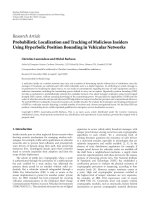
Figure 1: Illustration of CPA-based localization (a) 1D CPA localization, (b) 2D CPA localization.

gorithms applied on our energy-based localizer is also reported.
2.

EXISTING SOURCE LOCALIZATION METHODS

In a sensor network, a number of methods can be used to
locate and track a particular moving target. Some existing
methods are reviewed in this section.
2.1.

CPA-based localization method

In its original definition, a CPA (closest point of approach) point refers to the positions of two dynamically
moving objects at which they reach their closest possible
distance (see, />algorithm 0106/algorithm 0106.htm). In a sensor network
application, a CPA position is a point on the trajectory of a
moving target that is closest with respect to a stationary sensor node. Refer to Figure 1, using CPA point to estimate the
target location can be accomplished in two different ways.
(i) One-dimensional CPA localization: if a target is moving
along a road with known coordinates, the CPA point
with respect to a given sensor node is a coordinate on
this road that is closest to this observing sensor. Given
the sensor coordinate and the road coordinates, this
CPA point can be precomputed prior to operation. Assuming that the signal intensity will reach maximum
when a target is in the closest position, the time instant, when the target is on the CPA point, can be estimated from the time series observed at the sensor. Alternatively, the 1D CPA detection can be realized using
a tripped-wire style sensing modality, such as a polarized infrared (PIR) sensor.


Energy-Based Collaborative Source Localization

323

(ii) Two-dimensional localization: in a two-dimensional
sensor field, if the coordinate of the target trajectory
is not known in advance, the target position cannot
be precomputed. However, if the single intensity measured at neighboring sensors during the same time interval can be compared, the sensor which measures the
highest acoustic signal intensity should be the one that
is closest to the target. Then the location of that sensor
may be used as an estimate of the target location. This
is equivalent to the partition of the sensor field into N
Voronoi regions where N is the number of sensors. If
the target is in ith region, the corresponding ith sensor’s location will be used as an estimated location of
the target.
To use the CPA style localization method, it is desirable that
sufficient number of sensors are deployed within a given sensor field. Otherwise, the accuracy of the localization results
may be too coarse to yield less accurate results.
2.2. Target localization based on time delay
estimation
Sound signal travels at a finite speed. The same signal reaches
sensors at different locations with different amount of delays.
Denote v to be the source signal propagation speed rs and
ri , respectively, to be the target location and ith sensor’s location, and ti to be the time lags experienced at ith sensor.
Then the time delay between the source and received signal
at sensor i is ti = |rs − ri |/v + ni , where ni is used to model a
random noise due to measurement error. While the absolute
value of ti cannot be measured without knowing the source
location rs , the relative time delay measured with respect to a
reference sensor r0 can be measured as
v ti − t0 = vti = rs − ri − rs − r0 + ni .

(1)

Given N + 1 sensors, N equations like (1) can be formulated.
Then, one may estimate the unknown parameters v and rs
using maximum likelihood estimation [6, 10, 14, 20].
Alternatively, (1) can be expressed as
− 2 ri − r0

T

ri − r0

2

− 2 ti − t0

T
= ai x = ti − t0

2

x

= bi ,

1 ≤ i ≤ N,

(2)

where x = [(rs − r0 )T 1/ |v|2 |rs − r0 |/v]T is a (d + 2) × 1 vector
with d being the dimension of the sensor and target location vector. Note that elements of x are interdependent. With
N + 1(> d + 2) sensors, the target location can be found by

solving a constrained quadratic optimization problem: find x
to minimize C = Ax − b 2 subject to
d

xd+1 ·
i=1

2
xi2 = xd+2 ,

(3)

where A = [a1 a2 · · · aN ]T and b = [b1 b2 · · · bN ]T . The constraint described by (3) is due to the interdependent relations

between elements of the x vector. The target location can be
estimated as rs = r0 +[x1 · · · xd ]T , and the propagation speed
√
can be solved simultaneously as v = 1/ xd+1 . If constraint
(3) is ignored, one would need only to solve an overdetermined linear system Ax = b using the least square method
[9]. This method has also been refined using iterative improvement method and the Cram´ r-Rao bound of parame
eter estimation error has been derived [20]. Time-delayed
estimation-based source localization methods require accurate estimation of time delays between different sensor
nodes. To measure the relative time delay, acoustic signatures
extracted from individual sensor node must be compared. In
the extreme case, this will require the transmission of the raw
time series data that may consume too much wireless channel
bandwidth. Alternative approaches include cross-spectrum
[8] and range difference method [21].
3.

ENERGY-BASED COLLABORATIVE SOURCE
LOCALIZATION ALGORITHM

Energy-based source localization is motivated by a simple
observation that the sound level decreases when the distance
between sound source and the listener becomes large. By
modeling the relation between sound level (energy) and distance from the sound source, one may estimate the source
location using multiple energy readings at different known
sensor locations.
3.1.

An energy decay model of sensor signal readings

When the sound is propagating through the air, it is known
that [15] the acoustic energy emitted omnidirectionally from
a sound source will attenuate at a rate that is inversely proportional to the square of the distance. To verify whether
this relation holds in a wireless sensor network system with a
sound generated by an engine, we conducted a field experiment. In the absence of the adverse conditions laid out in the
introduction above, the experiment data confirms that such
an energy decay model is adequate. Details about this experiment will be reported in Section 3.2.
Let there be N sensors deployed in a sensor field in which
a target emits omnidirectional acoustic signals from a point
source. The signal energy measured on the ith sensor over a
time interval t, denoted by yi (t), can be expressed as follows:
yi (t) = gi ·

s t − ti
r t − ti − r i

α

+ εi (t).

(4)

In (4), ti is the time delay for the sound signal propagates
from the target (acoustic source) to the ith sensor, s(t) is a
scalar denoting the energy emitted by the target during time
interval t; r(t) is a d × 1 vector denoting the coordinates of
the target during time interval t; ri is a d × 1 vector denoting
the Cartesian coordinates of the ith stationary sensor; gi is the
gain factor of the ith acoustic sensor; α(≈ 2) is an energy decay factor, and εi (t) is the cumulative effects of the modeling
error of the parameters gi , ri , and α and the additive observation noise of yi (t). In general, during each time duration t,


324

EURASIP Journal on Applied Signal Processing

many time samples are used to calculate one energy reading
yi (t) for sensor i. Based on the central limit theorem, εi (t)
can be approximated well using a normal distribution with a
positive mean value, denoted by, say, µi (> 0), that is no less
than the standard deviation (STD) of the background measurement noise during that time interval. The STD of εi (t)
may also be empirically determined.
3.2. Experiment that validates the acoustic energy
decay model

3.3. Maximum likelihood parameter estimation
Assume that εi (t) in (4) are independent, identically distributed (i.i.d.) normal random variables with known mean

µi (> 0) and known variance σi2 , then each yi (t) will be an
i.i.d. conditional normal random variable with a probability
density function N(gi s(t)/ |r(t) − ri |α +µi , σi2 ). We also assume
that the time delay discrepancies among sensors are negligible, that is, ti = 0. Then, the likelihood function or, equivalently, the conditional joint probability can be expressed as
follows:
s(t), r(t)

i=0

1.4
1.2
1
0.8
0.6

To validate the model described in (4), we conducted a field
experiment. We used a lawn mower at stationary position as
our acoustic energy source. Two sensor nodes with acoustic microphone used in a DARPA SensIT project are placed
at different distances (5 m, 10 m, 15 m, 20 m, 25 m, 30 m)
away from the energy source. The microphones are placed
at about 50 cm above the ground and face the energy source.
The weather is clear with gentle breeze, and the temperature
is about 24 ◦ C.
The time series of both the acoustic sensors was recorded
at a sampling rate of 4960.32 Hz. Then the energy readings
were computed offline as the moving average (over a 0.5second sliding window) of the squared magnitude of the time
series. These energy readings then were fitted to an exponential curve to determine the decaying exponent α, as shown in
Figure 2.
For both acoustic sensors, within the 30-meter range, the
acoustic energy decay exponents are α = 2.1147 (with mean

square error 0.054374) and α = 2.0818 (with mean square error 0.016167), respectively. This validates the hypothesis that
the acoustic energy decreases approximately as the inverse of
the square of the source sensor distance.
We here assume α to be constant, which is valid if the
sound reverberation can be ignored and the propagation
medium (air) is roughly homogenous (i.e., no gusty wind)
during the process of experiment.

= f y0 (t), . . . , yN −1 (t) | σ 2 , {s(t), r(t)}


 1 N −1  y (t) − µ − g s(t)/ r(t) − r
i
i
i
i
∝ exp −
 2

σi2

0.4
0.2
0


2 


.

(5)
The objective of the maximum likelihood estimation is to
find the source energy reading and the source locations

0

5

10

15

20

25

30

Lawn mower, sensor 1, exponent = 2.1147

2

1.5

1

0.5

0

0

5

10

15

20

25

30

Figure 2: Acoustic energy decay profile of the lawn mower and the
exponential curve fitting.

{s(t), r(t)} to maximize the likelihood function. Since we as-

sume that the mean µi and the variance σi2 of εi (t) are known,
this is equivalent to minimizing the following log-likelihood
function:


L s(t), r(t) ∝

N −1 
i =0

yi (t) − µi − gi s(t)/ r(t) − ri

σi2



α 2



.

(6)
Given { yi (t), gi , ri , µi , σi2 ; 0 ≤ i ≤ N − 1} and α, the goal
is to find s(t) and r(t) to minimize L in (6). This can be accomplished using a standard nonlinear optimization method
such as the Nelder-Mead simplex (direct search) method implemented in the optimization package in Matlab.
3.4.

α

Lawn mower, sensor 2, exponent = 2.0818

1.6

Energy ratio and target location hypersphere

In the above formulation, we solve for both the source location r(t) and source energy s(t). In this section, we present
an alternative approach that is independent of the source energy s(t). This is accomplished by taking ratios of the energy
readings of a pair of sensors in the noise-free case to cancel
out s(t). We refer to this approach as the energy ratio formulation.

Energy-Based Collaborative Source Localization

325
So far, we have established that using the ratio of energy readings at a pair of sensors, the potential target location can be
restricted to a hypersphere whose center and radius are functions of the energy ratio and the two sensor locations. If more
sensors are used, more hyperspheres can be determined. If all
the sensors that receive the signal from the same target are
used, the corresponding target location hyperspheres must
intersect at a particular point that corresponds to the source
location. This is the basic idea of the energy-based source localization. Note that since the source energy is cancelled during the energy ratio computation, this method will not be
affected even if the source energy levels vary dramatically between successive energy integration time intervals.

4
3
2
1
κ = 0.8

0

κ = 0.6
κ = 0.7

κ = 0.4

−1
−2
−3

−4
−8

−6

−4

−2

3.5.

0

Figure 3: Two sensors are located at (−1, 0) and (1, 0). Four κ values
are used 0.4, 0.6, 0.7, and 0.8. The corresponding target location
circles and their centers are also shown.

Approximating the additive noise term εi (t) in (4) by its
mean value µi , we can compute the energy ratio κi j of the ith
and the jth sensors as follows:
κi j :=

−1/α

yi (t) − µi / y j (t) − µ j
gi (t)/g j (t)

r(t) − ri
=
. (7)

r(t) − r j

Note that for 0 < κi j = 1, all the possible source coordinates r(t) that satisfy (7) must reside on a d-dimensional
hypersphere described by the equation
r(t) − ci j

2

= ρi2j ,

(8)

where the center ci j and the radius ρi j of this hypersphere
associated with sensor i and j are given by
ci j =

ri − κi2j r j
,
1 − κi2j

ρi j =

κi j ri − r j
.
1 − κi2j

(9)

For convenience, we will call this hypersphere a target location hypersphere. When d = 2, such a hypersphere is a circle. When d = 3, it is a sphere. In Figure 3, several examples
corresponding to d = 2 and κi j < 1 are illustrated. As κi j increases, that is, as y j (t)/g j (t) → yi (t)/gi (t), the center of the

circle moves away from the sensors, and the radius increases.
In the limiting case when κi j → 1, the solution of (7)
form a hyperplane between ri and r j
r(t) · ri − r j =

ri

2

− rj

2

or equivalently,

2
r(t) · γi j = ξi j ,

(10)

where
γi j = ri − r j ,

ξi j =

ri

2

− Rj

2

2

.

(11)

Single target localization using multiple energy
ratios and multiple sensors

Suppose that N acoustic sensors detected the source signal emitted from a target during the same time intervals,
N(N − 1)/2 pairs of energy ratios can be computed. Based
on M (≤ N(N − 1)/2) these sensor energy ratios, our objective is to estimate the target location r(t) during that time
interval. Using a least square criterion, this problem leads to
a nonlinear least square optimization problem where the cost
function is defined as
M1

J(r) =

r − cm − ρm

2

M2

+

m=1

n=1

2

T
γn r − ξn ,

(12)

M1 + M2 = M,
where m and n are indices of the energy ratios computed
between different pairs of sensor energy readings, M1 is the
number of hyperspheres, and M2 is the number of hyperplanes. In practice, when |1 − κi2j | becomes too small, it may
cause numerical problem when evaluating r and ρ using (9).
In this case, the hyperplane equation (10) should be used instead. In our simulation, a value of 10−3 was set as the threshold to switch between these two type of error terms.
Note that if two sensors are both close to the target,
their energy readings have higher SNRs. Therefore, the energy ratio κi j computed from these energy readings will be
more reliable than that computed from a pair of sensors far
away from the target. Using the energy decay model, we may
use the relative magnitudes of energy readings as an indication of the target-sensor distance. As such, the error term in
(12) that correspond to sensors with higher-energy readings
should be given more weight than sensors that have lowerenergy readings.
Statistically, to employ the least square formulation in
(12), one must assume that both the hypersphere estimation error r − cm − ρm and the hyperplane estimation error
T
γn r − ξn are linear, independent Gaussian random variables
with zero mean and identical variance. Obviously, such an
assumption may not be true in practice and hence may cause

some performance degradation.
The cost function in (12) is nonlinear with respect to the
source location vector r. In this work, we experimented with
three nonlinear optimization methods to solve for r.


326

EURASIP Journal on Applied Signal Processing

(a) Exhaustive search over grid points within a predefined search region in the sensor field. This approach is the
most time consuming, yet most simple to implement. The
grid size determines the accuracy of the results.
(b) Multiresolution search. First a coarse-grained exhaustive search is conducted to identify likely source locations. Then a detailed fine-grained search is performed to refine the localization estimate.
(c) Gradient-based steepest descent search method.
Based on an initial source location (perhaps the previously
estimated position in the last time interval), say r(0), perform the following iteration:
r(k + 1) = r(k) − µ∇r J(r).

(13)

The gradient of J(r) can be expressed as
M1

∇J(r)2
m=1

r − cm
r − cm

ui j =

r − cm − ρm + 2

n=1

T
γn γn r − ξn .

(14)
In addition to the above methods, other standard optimization algorithms, such as the quasi-Newton’s method, conjugate gradient search algorithm, and many others can be used.
For comparison purpose, in the simulation, we also apply the
Nelder-Mead (direct search) method implemented in Matlab
optimization toolbox to minimize J(r).
In summary, there are two different methods to solve the
energy-based, (single) source localization problem.
(1) Direct minimization of the nonlinear log-likelihood
function L as in (7). With a number of acoustic energy measurements, this method is capable of simultaneously estimating the source location r(t) as well as the source energy s(t),
and the energy decay parameter α.
(2) Direct minimization of the cost function defined in
(12). A potential advantage of this method is that N(N − 1)/2
pairs of energy ratios can be used for the localization purpose
rather than the N energy readings used for minimizing the
likelihood function.

M1

jLinear (r) =
m=1

Consider two hyperspheres based on (8)
r(t) − ci0

2

2
= ρi0 ,

r(t) − c j0

2

= ρ2 .
j0

(15)

They are formed from the sensor pairs (i, 0) and ( j, 0).
Subtract each side and cancel the term |r(t)|2 , we have a
hyperplane equation
2
2
2 ci0 − c j0 r(t) = ci0 − ρi0 − c2 − ρ2 .
j0
j0

(16)

Substitute the definition in (9), the above equation is simplified to
ui j r(t) = θi j

which is a linear hyperplane equation with

(17)

ri

2

1 − κi2

−

2

rj

1 − κ2
j

.

(18)

uT r − θn
n

2

M2

+
n=1

2

T
γn r − ξn .

(19)

Note that there is no constraint imposed in (19). Given the
coefficients, a solution of r can be found in closed form.
4.

IMPLEMENTATION CONSIDERATIONS
Preprocessing: node and region energy detection

In a microsensor network, multiple acoustic sensors are deployed in a sensor field. Sensors within the same geographical region will form a group. One sensor node in a group
will be designated as a manager node where the collaborative
energy-based source localization will be performed.
During operation, individual sensor nodes will perform
energy-based target detection algorithm. For example, a constant false alarm rate (CFAR) detection algorithm [22, 23]
can be applied. Pattern classifiers may also be used to identify
the type of a detected target based on its acoustic or seismic
signatures.
Upon detection of a potential target, the sensor node
will report the finding to the manager node in the region. If
the number of detections reported by sensors within the region exceeds a predefined threshold, the manager node then
decides that a target is indeed detected by the region. This
implements a simple voting-based detection fusion within

the region. Only after a region-wide detection is confirmed,
the manager node will proceed to perform energy-based
source localization. Since the energy is computed on individual nodes, there is no need to recompute the acoustic energy
readings at the manager node.
4.2.

3.6. Unconstrained least square formulation

θi j =

Then, the cost function in (12) can be replaced by a linear
least square cost function

4.1.
M2

2r j
2ri
,
2 −
1 − κi
1 − κ2
j

Minimum number of collaborating sensors and
number of energy ratios used

In general, given N sensors, at maximal N(N − 1)/2 pairs of
energy ratios can be computed, and equal number of target
location hyperspheres (including some hyperplanes) can be

determined accordingly. The target location is the unique intersection of all these target location hyperspheres if the energy readings do not contain any measurement noise.
However, many of these relationships are actually redundant. In order to uniquely identify a single target location, in
this section, we want to determine (i) the constraint on the
sensor location configuration; and (ii) the minimum number of sensors required in theory to arrive at a unique source
location estimate. Regarding sensor location configuration,
we have the following results.
Lemma 1. Denote d to be the dimensionality of the sensor coordinate ri . If all N sensors locate on a subspace with a dimension


Energy-Based Collaborative Source Localization

327

d < d, then the centers of every target location hyperspheres
must lie within the same subspace.
Proof. From (10), since ci j is a linear combination of sensor
coordinates ri and r j , it must lie within the same subspace as
ri and r j . Hence this lemma is proved.
Specifically, in a 2D (d = 2) sensor field, if all sensors locate on a straight line, then all the centers of the corresponding target location circles must locate on the same straight
line. Since circles with their centers locating on the same
straight line cannot have a single point as their intersection
(either no intersection, or two or more points in the intersection), it is impossible to uniquely determine the target location. The exception is when the target location is also on
the same straight line. In a 3D (d = 3) sensor field, if all sensors locate on the same plane, then all the centers of the corresponding target location spheres must locate on the same
plane as well. Since spheres with their centers locating on the
same plane cannot intersect at just a single point in general,
it cannot uniquely determine the target location. Similarly,
the exception is when the target locates on the same plane.
These observations lead to the theorem below which is stated
without proof.
Theorem 1. In order to estimate a unique target location, not

all the sensors should be placed on a subspace whose dimension
is smaller than that of the sensor field unless the target location
is restricted in the same subspace as well.
Next, we consider the question of the minimum number
of sensors needed to locate a single target.
Lemma 2. Given three arbitrary placed sensors (say, 1, 2, and
3) in a 2D sensor field, the centers of every target location circles
c12 , c23 , and c31 must lie on the same straight line. Moreover, the
corresponding three target location circles may intersect at two
points if the target does not locate on the same straight line, or
at exactly one point if the target does locate on the same straight
line.
Proof. Performing linear combination of c12 and c23 in order
to eliminate r2 and using the relations κ12 κ23 κ31 = 1, one has
2
1 − κ12
2
c12 + 1 − κ23 c23
2
κ12
2
2
1 − κ12 r1 − κ12 r2
=
2
2
κ12
1 − κ12
2
+ 1 − κ23

2
r2 − κ23 r3
2
1 − κ23

r1
2
2 − κ23 r3
κ12
2 2
2
= κ23 κ31 r1 − κ23 r3
=

2
2
= −κ23 1 − κ31

(20)
2
r3 − κ31 r1
2
1 − κ31

2
2
= −κ23 1 − κ31 c31

=

2 2
1 − κ12 κ23
c31 .
2
κ12

But
2
2 2
1 − κ12 κ23
1 − κ12
2
+ 1 − κ23 =
.
2
2
κ12
κ12

(21)

Since c31 = βc12 + (1 − β)c23 , c12 , c23 , and c31 must lie on
the same straight line, next, note that the true target location
must be a point in each of the three corresponding target
location circles. In addition, three circles with their centers
located on the same straight line can intersect at most two
points, or not to intersect at all. Hence, these three circles
must intersect at exactly two points. When the target locates
on the same straight line where the centers of these circles locate, the two points of their intersection collide into a single

point. Hence, this lemma is proved.
Lemma 2 implies that, even though three sensors are not
on the same straight line, the centers of the corresponding target location circles (or spheres) still lie on the same
straight line. Using the argument in the proof of Theorem 1,
clearly three sensors are insufficient to estimate a unique target location in a 2D sensor field. It appears that at least four
sensor energy readings will be needed.
Lemma 2 addresses the 2D sensor field case. It can easily
be generalized to the 3D sensor field case.
Lemma 3. Given four arbitrary placed sensors in a 3D sensor field, the centers of every target location spheres must lie on
the same plane. Moreover, the six corresponding target location
spheres may intersect at two points if the target does not locate
on the same plane. Otherwise, their intersection contains exactly one point if the target also locates on the same plane.
Proof. Label these four sensors from 1 to 4. With four sensor
energy readings, six energy ratios can be computed. Using
Lemma 2, we conclude that
(i) c12 , c13 , and c23 must reside on the straight line La ;
(ii) c12 , c14 , and c24 must reside on the straight line Lb ;
(iii) c13 , c14 , and c34 must reside on the straight line Lc .
Lines La and Lb share the same point c12 . Hence, they must
lie on the same plane. Line Lc share one point to each line
La (c13 ) and line Lb (c14 ), respectively. Therefore, Lc must lie
on the same plane as La and Lb . The intersection regions between spheres with centers on La , Lb , and Lc , respectively, are
circles, respectively. With three circles in a 3D space, their
intersection contains at most two points. If the target also locates on the same plane, then these two points collide into
one.
Lemma 2 also reveals the redundancy among different
energy ratios. This critical observation can be stated as a
corollary as follows.
Corollary 1. Given energy ratios κ1i and κ1 j , the energy ratio
κi j is redundant and can be removed without affecting the solution of the target location.

328
Proof. Since κ1i κi j κ j1 = 1. Using Lemma 2, the intersection
between the target location circle (sphere), corresponding to
κi j with any of the other two circles (spheres), will be identical to the intersection between the circles (spheres) corresponding to κ1i and κ j1 . Hence, the inclusion of target location circle (sphere) of κi j does not contribute to any new
information to refine the solution space. Therefore, it is redundant.
Corollary 1 naturally leads to an important result in this
section.
Lemma 4. Given K sensors in a sensor field, then at most K − 1
pairs of energy ratios are independent in that the target location
circles (or spheres) corresponding to remaining energy ratios do
not further reduce the intersection region formed by the K − 1
target location circles (or spheres) of those independent energy
ratios.

EURASIP Journal on Applied Signal Processing

1.5

1

0.5

0

Proof. Denote sensor #1 as a reference sensor. Then denote
{κ1i ; 2 ≤ i ≤ K } for the set of K − 1 independent energy
ratios. Any other energy ratio κ jk , 2 ≤ j, k ≤ K, j = k will
be redundant according to Corollary 1. Thus, this lemma is

proved. Note that the set of K − 1 independent energy ratios
is not unique and can be chosen differently.
Theorem 2. Using the energy-based target localization method, at least four sensors not locating on the same straight line
are required to locate a single target in a 2D sensor field; and at
least five sensors not all locating on the same plane are required
to locate a single target in a 3D sensor field.
Proof. In a 2D sensor field, at least 3 (= K − 1) circles are
needed to form a single point intersection. Thus, at least four
sensor energy readings are needed. In a 3D sensor field, the
intersection of two spheres is a circle. The intersection between a sphere and a circle consists of at least two points (if
the intersection exists). Therefore, at least 4 (= K − 1) spheres
are needed to yield a single point intersection. Thus the minimum number of sensor energy readings needed in a 3D sensor field is five.

Energy-based collaborative target localization

2

−0.5

0

Sensor locations
Target locations

0.5

1

1.5

Center of circle

Figure 4: Localization of the target (star) at (1, 1) position using four sensors (triangle). The centers of the circles are small circles. Three circles corresponding to three independent equations are
generated. These three circles intersect at the target position as predicted. Parameters used s(t) = 1, gi = 1, and α = 2.

Figure 4 shows a simulation of target localization in a 2D
sensor field using four sensors and three energy ratios.

and the averaged background noise level due to wind and
other natural or man-made sound. Furthermore, due to the
need of collaborative region detection, a target is not considered detected unless a certain number of sensors voted positive detection. Hence the area that a target may be detected
should be the intersection of a minimum number of sensors
receptive fields.
If a target’s movement is restrictive, such as along a road,
then the search area can further be restricted to those areas where the target is allowed to move. These additional restrictions will enhance the accuracy of the source localization
process.

4.3. Nonlinear optimization search parameters

4.3.2

In developing nonlinear optimization methods to minimize
the cost function, a few parameters must be set properly to
ensure the performance of this proposed algorithm.

Depending on the size of the potential target and its speed,
the required accuracy of localization may vary. For example,
for a target with a dimension (say, length of a truck) larger
than 5 meters, it would be meaningless to try to locate the target within a 1-meter grid. In addition, if the target is moving
more than 10 m/s (about 20 mph), and the time duration to

compute one energy reading is 0.5 second, then the ambiguity regarding the actual location of the target during this time
period will be at least 5 meters. In this situation, any attempt
to locate the target within 5 meters will not be meaningful.
Therefore, in practical implementation, one should choose
appropriate accuracy measure.

4.3.1 Search area
The region of the potential target location can often be determined in advance, based on prior information about the
target, the region to be monitored, and the sensor locations.
Since acoustic energy decays exponentially with respect to
distance, the receptive field of an acoustic sensor (microphone) is limited. This range can be estimated based on the
maximum acoustic energy the target of interests may emit,

Search accuracy


Energy-Based Collaborative Source Localization

329

4.3.3 Initial search location

5.1.

For gradient-based search algorithms and other greedy
search algorithms, the initial search position is important.
One way to select the initial target location estimate is to use
the sensor location where the energy reading is the maximum
among all other sensors. The heuristic is that if the sensor
receives higher energy, then the true target location will be

closer to that sensor. In a localize-and-track scenario, the future target location can be predicted based on its trajectory.
In that case, the most likely position of the target during the
present time window may be chosen as the initial search position.

In this simulation, we compare four different optimization
algorithms for a single target, acoustic source localization
problem. For this purpose, 20 sensors are uniform randomly
distributed in a 50-meter by 50-meter sensor field. The location of the target is assumed to be within this sensor field.
The objective function is the energy ratio cost function
shown in (12). Two different modes are chosen to implement
the cost function: in mode 0, N − 1 independent energy ratios
(N: number of sensors) are used to form the cost function.
In mode 1, all possible N(N − 1)/2 energy ratios (with many
redundant measurements) are used to form the cost function. The hypothesis is that with redundant measurements
included in the cost function, it may better withstand parameter perturbations.
The following four search algorithms are implemented.

4.4. Distributive implementation
This proposed EBL algorithm would require at least four
sensor readings in order to yield a unique target location. Therefore, when implemented in a distributive sensor network, the acoustic energy readings will have to be
reported to a centralized location to facilitate localization
processing. To be deployed into a distributed wireless sensor network, it is desirable that a decentralized implementation of this proposed algorithm can be devised. By “decentralized,” we hope to devise a computation scheme such
that
(i) not all the energy readings need to be reported a centralized fusion center;
(ii) not all the computation required to evaluate the cost
function (12) need to be carried out at a centralized
processing center.
This can be accomplished by noting that the cost function
in (12) consists of summation of independent square error
terms. Given a potential target location r, each of the square

error term can be evaluated within a sensor node as soon
as it computes the k value after receiving the acoustic energy reading at a neighboring sensor node. Hence, instead of
transmitting the raw energy reading to the fusion center, the
partially computed cost function can be transmitted instead.
This way, the task of computation can be evenly distributed
over individual sensors. This scheme, however, may increase
the amount of internode wireless communications due to the
need to pass around the partially computed cost function for
each search grid.
5.

PERFORMANCE ANALYSIS

A number of factors may affect the performance of the
energy-based target localization algorithm. Due to the nonlinear nature and the complexity of the model, an analytical expression is difficult to obtain and may not reveal the
respective impacts of individual factors on the overall performance. In this section, extensive simulation will be conducted to compare the effectiveness of different optimization
algorithms as well as the sensitivities of the location estimates
with respect to perturbations of various parameters of the
model.

Comparison of different search algorithms

(1) Nelder-Mead (simplex) direct search (DS) algorithm:
the initial source location is obtained by an exhaustive
search at a grid size of 5 meters by 5 meters. For each
new target location, the DS method will evaluate the
cost function 11 × 11 = 121 times, and the DS search
will require additional cost function evaluations.
(2) Grid-based exhaustive search (ES) with a single grid
size of 1 m × 1 m. To estimate a target location, the ES

method will evaluate the cost function 51 × 51 = 2601
times.
(3) Multiresolution (MR) search with three levels of resolution (grid sizes) at 5 meters (5×), 2 meters (2×), and
1 meter (1×), respectively. The number of cost function evaluations for each new target location equals to
11 × 11 + 6 × 6 + 3 × 3 = 166.
(4) Gradient descent (GD) search algorithm using the gradient expression shown in (13). The initial location is
determined by ES at a grid size of 5 meters by 5 meters. The step size µ = 0.05 and maximal steps = 200.
The number of cost function evaluations for each new
target location will be 11 × 11 = 121 times plus the
number of gradient search steps.
Provided that the local search steps using either DS or
gradient search is within 50 steps of either the DS or the
GD search method, then the three search algorithms DS,
MR, and GD will require approximately the same number of
cost function evaluations (∼170). On the other hand, the ES
method will require 15 times more cost function evaluations.
Four experiment configurations are designed to compare
these search methods. In each configuration, a known fixed
energy is emitting from the source. At each sensor, the received energy is computed according to the exponential energy decay model described in (4) with K = 1 and εi = 0
(SNR = ∞). Three parameters in this model will be perturbed in configurations #2 to #4, respectively, as shown in
Table 1. Configuration # 1 is the control experiment with
no parameter perturbation. In configuration #1, the energy
decay constant α is sampled from a uniform distribution
[2 − ∆α, 2 + ∆α] with ∆α = 0.5. In configuration #3, each
sensor’s location r is subject to a random perturbation of


330

EURASIP Journal on Applied Signal Processing

0.5
0.4
0.3
0.2
0.1
0
−0.1
−0.2
−0.3
−0.4
−0.5
8

Mean in x

0.2

dα

ctrl

dr

dg

0.1
0
−0.1
−0.2

Mean in y

ctrl

dα

dr

dg

−0.3
−0.4
−0.5

STD in x

STD in y
8

6

6

4

4

2

2

0

0
dα

ctrl

dr

dg

ctrl

DS, mode 0

ES, mode 0

MR, mode 0

DS, mode 1

ES, mode 1

dα

dr

dg

GD, mode 0

MR, mode 1

Figure 5: Mean and standard deviation (STD) of target location estimation bias using different search algorithms.

Table 1: Parameter settings for different configurations to compare
four optimization search algorithms.
Configuration #

∆α

∆r

1
2
3
4

0
0.5
0
0

0
0
1
0

Table 2: Mean and variance of four different optimization methods, averaged over four test conditions.

∆g
0
0
0
0.5

magnitude ±∆r (= ±1) in both the x and y coordinates. In
configuration #4, the sensor gain g is perturbed to vary between [1 − ∆g, 1 + ∆g] with ∆g = 0.5.
Each experiment will be repeated 500 times using a cost
function evaluated with mode 0 setting and another 500
times with a cost function evaluated, using the mode 1 setting. The mean and the STD of the estimation error on xand y-axis are summarized in Figure 5.
Averaged over the four different parameter settings listed
in Table 1, the mean and variance of each method in both
x and y directions are listed in Table 2. Using T-test, it is
found that the differences in terms of the mean values of the
position estimation errors among the four different search
methods are statistically insignificant. Hence, despite large
number of cost function evaluations, the ES method does
not offer significant benefit in terms of improving source
localization accuracy. Of course, this conclusion is conditioned on the practice implemented in this experiment to
conduct initial coarse-grained ES (at 5 meters resolution) before commencing the three local search algorithms, namely,

Mean-x
ES
MR
DS
GD

Var-x

Mean-y

Var-y

0.093925
0.082425
0.086488
0.074825

5.939293
6.242463
8.287125
3.145920

−0.042100

6.466883
6.671392
8.492783
3.343724

−0.030850
−0.053988

0.029475

MR, DS, and GD. Without this initial ES, these methods may
be trapped in a local minimum solution that yields much

larger position estimation error.
The simulation results can also be used to compare the
effectiveness of evaluating the cost function using mode #0
(using minimum number of N −1 energy ratios) versus mode
#1 (using maximum number of N(N − 1)/2 energy ratios)
configurations. The results are listed in Table 3.
When the gain variation results are included, mode #1
performs worse than mode #0. This is because the erroneous
energy reading will be used to compute N − 1 energy ratios
in the mode #1 configuration and only 1 energy ratio for the
mode #0 configuration. Hence the same amount of error on
a single sensor reading will have a bigger impact in mode #1
than mode #0. However, excluding the gain variation factor,
in general, mode #1 performs much better than mode #0.
This result indicates that gain calibration of microphone is
essential to the success of the energy-based source localization method presented in this paper. This point is also clearly
illustrated in Figure 5.


Energy-Based Collaborative Source Localization

331

Table 3: Comparison between mode #0 and mode #1 results, averaged over all the four different methods, with different parameter
variations.

Table 4: Parameter settings for the experiments to examine the localization to perturbation.
Configuration #

Include dg

Mean-x

Var-x

Mean-y

Mode-0
Mode-1

0.081675
0.091267

4.087787
9.244179

0.0216
−0.10443

Mean-x

Var-x

Mean-y

0.044933
0.001889

2.959709
0.573453

∆r

∆g

SNR (dB)

1
2
3
4
5
6
7
8
9
10
11
12
13
14
15

1×1
5×5
10 × 10
1×1
1×1
1×1
1×1

1×1
1×1
1×1
1×1
1×1
1×1
1×1
1×1

0
0
0
0.2
0.5
1
0
0
0
0
0
0
0
0
0

0
0
0
0
0

0
0.5
1
5
0
0
0
0
0
0

0
0
0
0
0
0
0
0
0
0.2
0.5
1
0
0
0

∞

Var-y

Mode-0
Mode-1

∆α

4.115982
10.0473

Exclude dg

Grid size

Var-y

0.048542
−0.00394

2.694365
0.107678

5.2. Sensitivity analysis to parameter perturbations
In the previous section, we compared the performance of
four different search methods. In this section, we will investigate how the accuracy of the energy-based source localization method will be affected by inaccurate measurements of
parameters or the presence of noise.

∞
∞
∞
∞

∞
∞
∞
∞
∞
∞
∞

20
10
0

5.2.1 Factors affecting localization accuracy
(a) Energy decay exponent α. Although we have conducted
preliminary experiment and determined that the acoustic energy decay exponent α is approximately 2. However, this result is obtained using a point, omnidirectional sound source
in a favorable environment where the breeze is gentle and the
temperature is mild. It is likely that this parameter may be
varied at different situations. Thus, it is important to understand how sensitive the localization result will be with respect
to inaccurate estimate of the value of α.
(b) Sensor coordinate measurement ri . Sensor coordinates
can be obtained using on board global positioning system
(GPS) readings if such a device is available. However, highly
accurate sensor location measurements would require longterm averaging of GPS readings and may consume extensive
battery power. It is necessary to study what will be the impact of sensor location inaccuracy on the accuracy of energybased target localization.
(c) Acoustic sensor gain measurement gi . Not all acoustic
sensors are identical. Different sensors may exhibit different
gain characteristics. Thus, it is crucial to calibrate the gain
factor of individual acoustic sensors. It is also important to
gauge the effect of gain calibration error on the target localization accuracy.
(d) Acoustic energy measurement—signal-to-noise ratio

(SNR). As discussed earlier, the acoustic energy is usually averaged over a predefined time window as the sum of squares
of acoustic time series data (with mean subtracted). Energy
readings estimated this way may contain the energy of the
background noise. Suppose that the noise time series is modeled as a white Gaussian random process, its energy should
have a χ 2 distribution. However, if the number of time samples within each time window is sufficiently large, using central limit theorem, the noise energy can be modeled with an
equivalent Gaussian random process. Note that although the
noise energy level is likely to be the same over neighboring
sensor nodes, the source energy measured at different sen-

sor nodes are different according to the energy decay model.
In fact, due to energy decay, the SNR reduces by a factor
of (a log10 |r − ri |) provided that the background noise energy levels at every sensor are the same. If α ≈ 2, this means
2 dB SNR reductions for every additional 10 meters distance.
Hence, the SNR, measured at a sensor that is 50 meters away
from the source, will be 10 dB less than the SNR measured at
1 meter from the same source.
5.2.2

Simulation method

In this experiment, 20 randomly located sensors are used to
locate a randomly placed target. Both are located within a
predefined sensor field. We use the ES algorithm to minimize the cost function. As listed in Table 4, 15 configurations are designed for this experiment. The first three configurations are designed to compare the effect of different grid
size for ES. Three grid resolutions 1 meter, 5 meters, and 10
meters are used. The purpose of configurations #4 to #6 is
to compare the algorithm sensitivity with respect to variations of exponential decaying factor α. The actual value of α
is randomly drawn from the interval [α − ∆α, α + ∆α] with
∆α = 0.2, 0.5, and 1. Configurations #7 to #9 are designed to
compare the effect of inaccurate sensor locations measurement. Each sensor location vector r is randomly perturbed
as r + ∆r where ∆r = [∆x, ∆y] and ∆x, ∆y are both random

variables uniformly distributed over an interval (in meters)
[−0.5, 0.5], [−1, 1], or [−5, 5]. In configurations #10 to #12,
we intend to examine the impacts of inaccuracy in acoustic
sensor gain variation. The actual sensor gain is drawn randomly from a uniform distribution [1 − ∆g, 1 + ∆g]. Our
aim in designing configurations #13 to #15 is to examine
the effects of different SNRs. The energy variations in these
configurations, specified in dB, are measured at 1 meter away
from the source. As we discussed earlier, the actual SNR at
each sensor varies, depending on the relative distance to the


332

EURASIP Journal on Applied Signal Processing
Table 5: Mean (bias) and STD of simulation results using different grid sizes.
Bias
(20, 19)
(10, 9)
(5, 4)
(20, 190)
(10, 45)
(5, 10)
STD
(20, 19)
(10, 9)
(5, 4)
(20, 190)
(10, 45)
(5, 10)

1 × 1 grid
0.041
0.009
0.01
−0.007
−0.006
−0.01
1 × 1 grid
0.7792
0.673
0.83
0.3036
0.3054
0.3307

x-coordinate
5 × 5 grid

10 × 10 grid

−0.0434

0.0649

0.0216
0.0516
0.0216
−0.0134
0.0366

−0.0451

x-coordinate
5 × 5 grid
2.7691
2.4047
2.5052
1.4664
1.5007
1.5853

1 × 1 grid

−0.0151

0.0576
0.0396
0.0316
0.0176
0.0166
0.0146

10 × 10 grid

1 × 1 grid

4.4097
4.0726
4.0247
3.0664

3.111
3.3359

0.7147
0.6453
0.721
0.296
0.2978
0.3151

0.1149
−0.1151
−0.1151

source. SNR = ∞ implies that there is no noise, that is, ε = 0.
SNR = 0 means that the noise energy is equal to that of the
source energy. The perturbations on r, g, and SNR are applied to all individual sensors.
As in the previous experiment, different numbers of sensors and numbers of energy ratios may affect the localization
accuracy. To better understand their impact, we devised six
different modes and denoted this combination, using a vector (N, M), where N = number of sensors used and M =
number of energy ratios used. These modes are (20, 19),
(10, 9), (5, 4), (20, 190), (10, 45), and (5, 10). In the first three
modes, M = N − 1. In the last three, M = N(N − 1)/2.
For each configuration and each of the mode, 1000 independent simulations are performed and the mean and STD of
the results in both x and y directions are computed for further analysis.
5.2.3 Results and discussions
(a) Different grid size (search resolution). The simulation results corresponding to configurations #1 to #3 are listed in
Table 5.
The following two observations are worth noting.
(i) Bias—the energy-based source localization method

yields unbiased estimate at each of the three grid sizes.
(ii) Variance—suppose that the target location is uniformly and randomly distributed within a grid, then
the expected STD of position estimation error will be
√
/ 12 ∼ 0.2887 at each x- and y-direction. From
=
Table 5, it is clear that when the maximum number of
energy ratios are used, that is, M = N(N − 1)/2, the
position estimation error will approximate this lower
bound. On the other hand, when M = N − 1, the
variances are uniformly larger. This is more prominent
when the grid size is small. Our conjecture is that the

y-coordinate
5 × 5 grid
0.1755
0.2005
0.0755
−0.0045
−0.0395
0.0305
y-coordinate
5 × 5 grid
2.7548
2.418
2.71
1.4916
1.5019
1.5612

10 × 10 grid
0.1615
0.0915
0.0115
−0.0285
0.0015
−0.1285
10 × 10 grid
4.2629
4.0569
4.2094
2.9337
2.9642
3.2578

cost functions formed, using N − 1 energy ratios does
not, have the same global minimum as the cost function formed using N(N − 1)/2 energy ratios.
(b) Variation on α—the results corresponding to configurations #1, 4, 5, and 6 are listed in Table 6.
Again, we make two observations on this table.
(i) Bias—the variation of the energy decay exponent α has
little effect on the bias of the estimation error.
(ii) STD—the variations of α did impact the results when
M = N − 1. It seems that the more sensors are used,
the larger the STD is. On the other hand, when M =
N(N − 1)/2, the variation of α as large as 1, that is, the
values of α varies between 1 and 3, has little effect on
the STD of the location estimation error. This is an important evidence to justify the use of a nominal value
of α = 2 provided the maximum number of energy
ratios is included in the cost function definition.
(c) Variations on sensor position error r—the results are

summarized in Table 7.
As in the previous cases, the sensor location errors will
not impose any bias to the location estimates. What is different from the previous cases is that the STD of estimation errors seem to be similar using either M = N − 1 or
M = N(N − 1)/2 energy ratios.
(d) Variations on sensor gain g—the results are summarized in Table 8.
Consistent with the results obtained in the previous experiment, the energy-based source localization algorithm is
quite sensitive to the error in gain calibration. In particular,
in terms of STD, two important trends can be observed from
Table 8.
(i) More sensors give worse results. Apparently, more sensors with wrong gain factor will impact significantly


Energy-Based Collaborative Source Localization

333

Table 6: Mean and STD of position estimate errors due to variation of α.
Bias

∆α = 0

(20, 19)
(10, 9)
(5, 4)
(20, 190)
(10, 45)
(5, 10)

0.041
0.009

0.01
−0.007
−0.006
−0.01

STD

∆α = 0

(20, 19)
(10, 9)
(5, 4)
(20, 190)
(10, 45)
(5, 10)

0.7792
0.673
0.83
0.3036
0.3054
0.3307

x-coordinate
∆α = 0.2
∆α = 0.5

∆α = 1

∆α = 0

−0.07

−0.0347

−0.2275

−0.086

−0.0047

−0.0875

−0.055

0.0593

−0.0395

0.004
0.003
0.004

−0.0177
−0.0027

0.0075
0.0035
0.0145

0.0576
0.0396
0.0316
0.0176
0.0166
0.0146

x-coordinate
∆α = 0.2
∆α = 0.5

∆α = 1

∆α = 0

2.9646
2.183
2.1823
0.2935
0.2979
0.3549

0.7147
0.6453
0.721
0.296
0.2978
0.3151

0.8585

0.7729
0.7788
0.3007
0.3037
0.3225

−0.0097

1.4971
1.1727
1.2808
0.2841
0.2833
0.3273

y-coordinate
∆α = 0.2
∆α = 0.5

∆α = 1

−0.0236

−0.0062

−0.0116

−0.0082

0.0279

0.0189
0.0229
0.0039
0.0099
0.0129

0.0104

−0.0252

−0.0026

−0.0072

−0.0046

−0.0002

−0.0076

−0.0002

y-coordinate
∆α = 0.2
∆α = 0.5

∆α = 1

0.9253
0.7842

0.8247
0.2993
0.2996
0.3259

1.4706
1.205
1.4049
0.2962
0.3007
0.3276

2.9502
2.1486
1.993
0.291
0.2898
0.3286

Table 7: Mean and STD of source location estimation error due to different sensor location errors.
Bias
(20, 19)
(10, 9)
(5, 4)
(20, 190)
(10, 45)
(5, 10)
STD
(20, 19)
(10, 9)

(5, 4)
(20, 190)
(10, 45)
(5, 10)

d(r) = 0
0.041
0.009
0.01
−0.007
−0.006
−0.01
d(r) = 0
0.7792
0.673
0.83
0.3036
0.3054
0.3307

x-coordinate
d(r) = 0.5
d(r) = 1

d(r) = 5

d(r) = 0

−0.0088

−0.0186

−0.0848

0.0232
0.0132
−0.0378

0.0074
0.0274
−0.0876
0.0154
0.1484

0.0576
0.0396
0.0316
0.0176
0.0166
0.0146

x-coordinate
d(r) = 0.5
d(r) = 1

d(r) = 5

d(r) = 0

3.5845

3.7525
4.093
4.8538
4.0243
3.9941

0.7147
0.6453
0.721
0.296
0.2978
0.3151

0.0245
0.0195
0.0505
0.0005
0.0185
0.0235

0.873
0.8418
1.061
0.3672
0.4718
0.8271

−0.0538

1.0054

1.0797
1.6229
0.5774
0.8653
1.5717

the shape of the cost function and therefore the location of its minimum.
(ii) Using M = N − 1 or M = N(N − 1)/2 yields approximately the same quality of the results. The favor is
slightly tilted toward the former. However, the difference is not statistically significant.
The key lesson learned from these three configurations is
that sensor gain calibration is crucial to the success of this algorithm. Hence, each sensor should be calibrated before deployment in the field.
(e) Variations on SNR—the results are summarized in
Table 9.

y-coordinate
d(r) = 0.5
d(r) = 1
0.0136
0.0586
0.0546
−0.0064
−0.0074
0.0176

−0.0121

d(r) = 5

0.0109
0.0829

−0.0211

0.1262
0.1362
−0.0088
0.0852
0.0092
−0.0978

y-coordinate
d(r) = 0.5
d(r) = 1

d(r) = 5

0.842
0.8391
1.1529
0.3664
0.4458
0.8392

0.0149
−0.0031

1.0074
1.0405
1.6245
0.5541
0.8016

1.7502

3.5751
3.594
4.4003
4.9591
3.8904
4.2185

The effect of additive background noise is similar to that
of sensor gain perturbation: both will affect the accuracy of
energy measurements at each sensor. From Table 9, one observes that
(i) the more sensors are used, the larger the STD. Apparently, the energy estimation errors do not cancel each
other when more sensor readings are used.
(ii) other than SNR = ∞, the two modes M = N − 1 and
M = N(N − 1)/2 yield approximately the same standard deviation. The differences increase when more
sensors are being used.
We must note that for practical vehicle target, the SNR at


334

EURASIP Journal on Applied Signal Processing
Table 8: Mean and STD of localization error for different sensor gain values.

Mean
(20, 19)
(10, 9)
(5, 4)
(20, 190)

(10, 45)
(5, 10)
STD
(20, 19)
(10, 9)
(5, 4)
(20, 190)
(10, 45)
(5, 10)

d(g) = 0
0.041
0.009
0.01
−0.007
−0.006
−0.01
d(g) = 0
0.7792
0.673
0.83
0.3036
0.3054
0.3307

x-coordinate
d(g) = 0.2
d(g) = 0.5
0.0869
0.0369

0.0619
0.1429
0.0519
0.0489

0.0152
−0.0058

0.0512
0.1452
0.1922
0.0292

x-coordinate
d(g) = 0.2
d(g) = 0.5
1.3112
1.5515
2.0879
2.9657
2.3371
2.2247

0.852
3.2465
3.213
7.4987
4.2964
3.3303

d(g) = 1

d(g) = 0

0.0727
0.0977
−0.0553
0.0217
0.1137
0.0067

0.0576
0.0396
0.0316
0.0176
0.0166
0.0146

d(g) = 1

d(g) = 0

9.0153
6.5942
4.9774
10.2708
6.0754
4.526

0.7147

0.6453
0.721
0.296
0.2978
0.3151

y-coordinate
d(g) = 0.2
d(g) = 0.5
0.0148
0.0268
−0.0582
0.0168
0.0808
−0.0022

0.0143
0.0043
0.0253
0.2463
0.1133
0.0233

y-coordinate
d(g) = 0.2
d(g) = 0.5
1.2086
1.5616
1.9148
2.7917

2.1831
2.1157

d(g) = 1
0.3178
0.1988
0.1958
0.5738
0.2618
0.2008
d(g) = 1

3.5631
3.1859
3.2588
7.0885
4.1489
3.3239

9.1049
6.3942
4.992
10.0506
5.9161
4.3258

y-coordinate
SNR = 20 dB
SNR = 10 dB

SNR = 0 dB

Table 9: Mean and STD of position estimation error due to background noise.
Mean
(20, 19)
(10, 9)
(5, 4)
(20, 190)
(10, 45)
(5, 10)
STD
(20, 19)
(10, 9)
(5, 4)
(20, 190)
(10, 45)
(5, 10)

SNR = ∞
0.041
0.009
0.01
−0.007
−0.006
−0.01
SNR = ∞
0.7792
0.673
0.83
0.3036

0.3054
0.3307

x-coordinate
SNR = 20 dB
SNR = 10 dB
−0.1776
−0.2166
−0.1146
−0.6146
−0.1546
−0.0896

0.1094
0.1604
0.1784
0.4334
0.3234
0.1784

x-coordinate
SNR = 20 dB
SNR = 10 dB
5.6954
3.8446
2.8921
10.9375
5.1254
3.0126

8.1004
5.6287
4.4332
12.6961
6.5798
4.5768

SNR = 0 dB

SNR = ∞

−0.082

−0.103

0.0576
0.0396
0.0316
0.0176
0.0166
0.0146

SNR = 0 dB

SNR = ∞

9.837
6.7225
5.2167
13.5552

7.2908
5.0284

0.7147
0.6453
0.721
0.296
0.2978
0.3151

0.08
−0.035
−0.202
−0.111

the source is often much higher than 40 dB. The condition of 0 dB or worse may occur when strong wind directly
blowing into a microphone without wind-damper protection, or the microphone is hit by blowing debris or similar
interferences.
5.2.4 Discussion
Based on the above two experiments, one may deduce the
following guidelines for the proper implementation of the
energy-based acoustic source localization algorithm:
(i) proper definition of the sensor field where the potential target localization will lie;

0.2093
0.1833
0.0243
0.2893
0.3033
−0.0397

0.0268
0.0228
−0.1152
−0.0312
−0.0822
−0.0312

y-coordinate
SNR = 20 dB
SNR = 10 dB
5.5849
3.9481
3.1086
10.9602
5.2017
3.1965

7.5979
5.2083
3.9147
12.4986
6.5202
4.1028

0.5168
0.2688
0.1878
0.7268
0.3788

0.1738
SNR = 0 dB
9.4387
6.4093
5.2041
13.3184
7.1348
4.9295

(ii) careful calibration of sensor gain factor;
(iii) use one of the fast search algorithm MR, GD, or simplex DS method after first conducting a coarse-grained
ES within the sensor field;
(iv) using few reliable energy readings from a few sensor
is preferred to using many unreliable energy readings
from more sensors. If one may assess the accuracy of
individual energy reading, it will be possible to prune
out unreliable sensor readings to enhance the overall
localization accuracy;
(v) using more energy ratios (i.e., M = N(N − 1)/2) often
yield more reliable results.


Energy-Based Collaborative Source Localization

335

Distribution of errors: EBL

300

Distribution of errors: CPA

300

200

200

100

100

0

0

−100

−100

−200

−200

−300
−300

−200

−100

0

100

200

300

EBL position error histogram

200

−300
−300

100

200

300

100

50

0

150

100

−100

2D CPA position error histogram

200

150

−200

50

0

0

100

200

300

0

0

100

200

300

Figure 6: Comparison between EBL and CPA localization method.

5.3. Comparison with other acoustic localization
methods
The energy-based single acoustic source localization method
presented above differs from other existing method in a
number of important aspects, as follows.
(1) Target positions are estimated at constant time interval—with the CPA-based approach, a new target location is obtained only when the moving target passes
through another sensor. If the target stopped and remain stationary for a period of time, no additional
CPA detection will be made. With energy-based source
localization method, as long as the target continue to
emit acoustic energy, its location will be estimated on
a regular time interval, even when the target vehicle is
idling and remain stationary. This significantly simplifies the task of the tracking algorithm.
(2) Energy-based method reduces communication requirements over wireless channels, and hence conserves
power—energy is a scalar quantity that is computed
over a number of data samples. The frequency of how

often an energy reading is computed can be easily adjusted to meet the performance requirement and communication bandwidth as well as energy consumption constraints. Time delay-based localization methods will require accurate estimate of relative time delays (or phase difference in frequency domain) between different sensors. Hence, they may require more
raw data samples or corresponding frequency components to be exchanged between sensor nodes.
We conducted a preliminary experiment comparing the
proposal EBL algorithm with the 2D CPA algorithm. A sensor field of 300 meters by 300 meters is deployed with eight
acoustic sensors at random locations. The target location is
also randomly chosen within the same sensor field. Both sensor locations and target locations are drawn from a uniform
distribution. The measured sensor locations, however, are assumed to suffer a measurement error that is uniformly distributed over [−0.5, 0.5] meters. The acoustic sensor gain g
is assumed to vary between 0.6 and 1.2 compared to a calibrated value of 1. Each sensor is also subject to a 20 dB

336

EURASIP Journal on Applied Signal Processing
Table 10: Mean and STD of the estimation error.
EBL

Mean value

−0.14873

−0.60246

STD

49.0514

46.5717

CPA
0.41733
48.292

−0.72433

A. D’Costa, and M. Duarte. The authors would also like to
extend their gratitude to the anonymous reviewers for their
very constructive and helpful comments. In particular, Sections 3.6, 4.4, and 5.3 are added upon their suggestions.

53.8862

REFERENCES
additive Gaussian random noise with zero mean. The source
energy level is fixed at a value of 1000.
For the 2D CPA method, the measured sensor location
corresponding to the sensor receiving maximum acoustic energy will be used as an estimate of the target location. For the
EBL method, a search grid of 10 meters, each side will be
used to enable an ES. The experiment contains 1000 independent trials. In each trial, the sensor locations, the target
location, the perturbations on sensor location measurement,
sensor gain variation, and additive noise are generated according to the specified distribution.
The mean and STDs of the target position estimation errors of these two methods are listed in Table 10.
The results are summarized in Figure 6. The ellipses in
the top row specify the covariance matrices of these errors
with each grey dot representing error incurred in a particular try. The histograms of the magnitudes of the position
estimation errors are depicted at the bottom row.
6.

DISCUSSION AND CONCLUSION

In this paper, we have presented the energy-based source localization algorithm, and derived theoretical results on the
number of sensors required to yield a unique location estimate. We have also conducted extensive simulation to compare different search algorithms and to study the parameter
sensitivity characteristics of this proposed algorithm.
An implicit advantage of this proposed algorithm is its
simplicity: only acoustic energy measured during a specific
period is needed. However, this simplicity also implies many
practical difficulties that need to be mitigated. In particular,
we note that the microphone gain calibration and SNR estimation are two key factors that affect the accuracy of this
proposed algorithm.
Currently, we are working to apply this algorithm to real

data obtained in the test ground. We are also studying potential extension of this algorithm to localize more than a single
target within the sensor field.
ACKNOWLEDGEMENTS
This work was partly supported by DARPA under Grant no.
F 30602-00-2-0555. The authors would like to thank Professors A. Sayeed, P. Ramanathan, K. Saluja at UW-Madison,
Prof. K. Yao, and Dr. R. E. Hudson at University of California,
Los Angles, for helpful discussions. The acoustic energy decay profile experiment is conducted with the assistance from
UW-Madison SensIT team graduate students K. C. Wang,
T. Chin, T. Clouquerur, V. Phipatanasuphcorn, A. Ashraf,

[1] D. Estrin, L. Girod, G. Pottie, and M. Srivastava, “Instrumenting the world with wireless sensor networks,” in Proc. IEEE
Int. Conf. Acoustics, Speech, Signal Processing, Salt Lake City,
Utah, USA, May 2001.
[2] C. Savarese, J. M. Rabaey, and J. Beutel, “Locationing in
distributed Ad-hoc wireless sensor networks,” in Proc. IEEE
Int. Conf. Acoustics, Speech, Signal Processing, Salt Lake City,
Utah, USA, May 2001.
[3] N. L. Owsley, “Sonar array processing,” in Array Signal Processing, S. Haykin, Ed., pp. 115–193, Prentice-Hall, Englewood
Cliffs, NJ, USA, 1985.
[4] A. Tolstoy, Matched Field Processing for Underwater Acoustics,
World Scientific Publications, Singapore, 1993.
[5] M. S. Brandstein, J. E. Adcock, and H. F. Silverman, “A
localization-error-based method for microphone-array design,” in Proc. IEEE Int. Conf. Acoustics, Speech, Signal Processing, Atlanta, Ga, USA, May 1996.
[6] M. S. Brandstein, J. E. Adcock, and H. F. Silverman, “A closedform location estimator for use with room environment microphone arrays,” IEEE Trans. Speech, and Audio Processing,
vol. 5, no. 1, pp. 45–50, 1997.
[7] J. Huang, N. Ohnishi, and N. Sugie, “Sound localization in reverberant environment based on the model of the precedence
effect,” IEEE Trans. Instrumentation and Measurement, vol. 46,
no. 4, pp. 842–846, 1997.
[8] M. Omologo and P. Svaizer, “Acoustic source location in
noisy and reverberant environment using CSP analysis,” in

Proc. IEEE Int. Conf. Acoustics, Speech, Signal Processing, Atlanta, Ga, USA, May 1996.
[9] K. Yao, R. E. Hudson, C. W. Reed, D. Chen, and F. Lorenzelli,
“Blind beamforming on a randomly distributed sensor array
system,” IEEE Journal on Selected Areas in Communications,
vol. 16, no. 8, pp. 1555–1567, 1998.
[10] C. W. Reed, R. Hudson, and K. Yao, “Direct joint source localization and propagation speed estimation,” in Proc. IEEE
Int. Conf. Acoustics, Speech, Signal Processing, Phoenix, Ariz,
USA, May 1999.
[11] S. Haykin, J. H. Justice, N. L. Owsley, J. L. Yen, and A. C. Kak,
Array Signal Processing, Prentice-Hall, Englewood Cliffs, NJ,
USA, 1985.
[12] G. C. Carter, Coherence and Time Delay Estimation, IEEE
Press, Mill Road Edison, NJ, USA, 1993.
[13] “Special issue on time-delay estimation,” IEEE Trans. Acoustics, Speech, and Signal Processing, vol. 29, June 1981.
[14] J. O. Smith and J. S. Abel, “Closed-form least-squares location estimation from range-difference measurements,” IEEE
Trans. Acoustics, Speech, and Signal Processing, vol. 35, no. 12,
pp. 1661–1669, 1987.
[15] L. Kinsler, A. Frey, A. Coppens, and J. Sanders, Fundamentals
of Acoustics, John Wiley and Sons, New York, NY, USA, 1982.
[16] K. Srodecki, “Evaluation of the reverberation decay quality in
rooms using the autocorrelation function and the cepstrum
analysis,” Acustica, vol. 80, no. 3, pp. 216–225, 1994.
[17] Y. L. Li, M. J. White, and S. J. Franke, “New fast field programs for anisotropic sound propagation through an atmosphere with a wind velocity profile,” Journal of the Acoustical
Society of America, vol. 95, pp. 718–726, 1994.


Energy-Based Collaborative Source Localization
[18] E. M. Salomons, “Downwind propagation of sound in an atmosphere with a realistic sound-speed profile: a semianalytical ray model,” Journal of the Acoustical Society of America,
vol. 95, no. 5, pp. 2425–2436, 1994.
[19] T. Watanabe and S. Yamada, “Sound attenuation through absorption by vegetation,” Journal of the Acoustical Society of

Japan, vol. 17, pp. 175–182, 1996.
[20] J. C. Chen, R. E. Hudson, and K. Yao, “A maximum likelihood
parametric approach to source localization,” in Proc. IEEE
Int. Conf. Acoustics, Speech, Signal Processing, Salt Lake City,
Utah, USA, May 2001.
[21] J. O. Smith and J. S. Abel,
“The spherical interpolation method for closed-form passing source localization
using range difference measurements,”
in Proc. IEEE
Int. Conf. Acoustics, Speech, Signal Processing, Dallas, Tex,
USA, 1987.
[22] R. E. Schwartz, “Minimax CFAR detection in additive Gaussian noise of unknown covariance,” IEEE Transactions on Information Theory, vol. 15, pp. 722–725, 1969.
[23] J. Dabkowski Jr., “CFAR operation in non-homogeneous and
point clutter,” in Proc. National Electronics Conference, 1970.
Dan Li received the B.S.E.E. degree from Tsinghua University, Beijing, China, in 1996;
the M.S. degree in biomedical engineering
from the University of Kentucky in 1999;
and the M.S.E.E. degree from the University
of Wisconsin-Madison in 2001. He is currently a Researcher and Development Engineer at the Guidant Corporation, St. Paul,
Minn, USA. His research interests are in algorithm development and applications of
DSP and statistical signal processing.
Yu Hen Hu received the B.S.E.E. degree
from National Taiwan University, Taiwan,
in 1976. He received the M.S. and Ph.D.
degrees both in electrical engineering from
University of Southern California, Los Angeles, Calif in 1980 and 1982, respectively.
Currently, he is a Professor at the Electrical
and Computer Engineering Department of
the University of Wisconsin-Madison, Wis,
USA. Previously, he has been with the Electrical Engineering Department of the Southern Methodist University, Dallas, Tex, USA. Dr. Hu’s research interests include multimedia signal processing, design methodology and implementation of

signal processing algorithms and systems, sensor network and distributive signal processing algorithms, and neural network signal
processing. He published more than 200 journal and conference
papers and edited two books: Programmable Digital Signal Processors and Handbook of Neural Network Signal Processing. Dr. Hu is
a Fellow of IEEE. He served as Associate Editor for IEEE Transactions on Signal Processing, IEEE Signal Processing Letters, Journal of VLSI Signal Processing, EURASIP Journal on Applied Signal
Processing. He served as Secretary of IEEE signal processing society, board of governors of IEEE neural network council, Chair of
IEEE signal processing society, and neural network signal processing technical committee.

337