Báo cáo hóa học: "Research Article Probabilistic Localization and Tracking of Malicious Insiders Using Hyperbolic Position Bounding in Vehicular Networks" pot

Hindawi Publishing Corporation
EURASIP Journal on Wireless Communications and Networking
Volume 2009, Article ID 128679, 13 pages
doi:10.1155/2009/128679
Research Article
Probabilistic Localization and Tracking of Malicious Insiders
Using Hyperbolic Position Bounding in Vehicular Networks
Christ ine Laurendeau and Michel Barbeau
School of Computer Science, Carleton University, 1125 Colonel By Drive, Ottawa, ON, Canada K1S 5B6
Correspondence should be addressed to Christine Laurendeau,
Received 12 December 2008; Accepted 1 April 2009
Recommended by Shuhui Yang
A malicious insider in a wireless network may carry out a number of devastating attacks without fear of retribution, since the
messages it broadcasts are authenticated with valid credentials such as a digital signature. In attributing an attack message to
its perpetrator by localizing the signal source, we can make no presumptions regarding the type of radio equipment used by a
malicious transmitter, including the transmitting power utilized to carry out an exploit. Hyperbolic position bounding (HPB)
provides a mechanism to probabilistically estimate the candidate location of an attack message’s originator using received signal
strength (RSS) reports, without assuming knowledge of the transmitting power. We specialize the applicability of HPB into the
realm of vehicular networks and provide alternate HPB algorithms to improve localization precision and computational efficiency.
We extend HPB for tracking the consecutive locations of a mobile attacker. We evaluate the localization and tracking performance
of HPB in a vehicular scenario featuring a variable number of receivers and a known navigational layout. We find that HPB can
position a transmitting device within stipulated guidelines for emergency services localization accuracy.
Copyright © 2009 C. Laurendeau and M. Barbeau. This is an open access article distributed under the Creative Commons
Attribution License, which permits unrestricted use, distribution, and reproduction in any medium, provided the original work is
properly cited.
1. Introduction
Insider attacks pose an often neglected threat scenario when
devising security mechanisms for emerging wireless tech-
nologies. For example, traffic safety applications in vehicular
networks aim to prevent fatal collisions and preemptively
warn drivers of hazards along their path, thus preserving

numerous lives. Unmitigated attacks upon these networks
stand to severely jeopardize their adoption and limit the
scope of their deployment.
The advent of public key cryptography, where a node
is authenticated through the possession of a public/private
key pair certified by a trust anchor, has addressed the
primary threat posed by an outsider without valid cre-
dentials. But a vehicular network safeguarded through a
Public Key Infrastructure (PKI) is only as secure as the
means implemented to protect its member nodes’ private
keys. An IEEE standard has been proposed for securing
vehicular communications in the Dedicated Short Range
Communications Wireless Access in Vehicular Environments
(DSRC/WAVE) [1]. This standard advocates the use of digital
signatures to secure vehicle safety broadcast messages, with
tamper proof devices storing secret keys and cryptographic
algorithms in each vehicle. Yet a convincing body of
existing literature questions the resistance of such devices
to a motivated attacker, especially in technologies that are
relatively inexpensive and readily available [2, 3]. In the
absence of strict distribution regulations, for example, if
tamper proof devices for vehicular nodes are available off
the shelf from a neighborhood mechanic, a supply chain
exists for experimentation with these devices for the express
purpose of extracting private keys. The National Institute
of Standards and Technology (NIST) has established a
certification process to evaluate the physical resistance of
cryptographic processors to tampering, according to four
security levels [4]. However, tamper resistance comes at
a price. High end cryptographic processors certified at

the highest level of tamper resistance are very expensive,
for example, an IBM 4764 coprocessor costs in excess
of 8000 USD [5]. Conversely, lower end tamper evident
cryptographic modules, such as smartcards, feature limited
mechanisms to prevent cryptographic material disclosure
2 EURASIP Journal on Wireless Communications and Networking
or modification and only provide evidence of tampering
after the fact [6]. The European consortium researching
solutions in vehicular communications security, SeVeCom,
has highlighted the existence of a gap in tamper resistant
technology for use in vehicular networks [7]. While low
end devices lack physical security measures and suffer from
computational performance issues, the cost of high end
modules is prohibitive. The gap between the two extremes
implies that a custom hardware and software solution is
required, otherwise low end devices may be adopted and
prove to be a boon for malicious insiders.
Vehicle safety applications necessitate that each network
device periodically broadcast position reports, or beacons.
A malicious insider generating false beacons whose digital
signature is verifiable can cause serious accidents and
possibly loss of life. Given the need to locate the trans-
mitter of false beacons, we have put forth a mechanism
for attributing a wireless network insider attack to its
perpetrator, assuming that a malicious insider is unlikely
to use a digital certificate linked to its true identity. Any
efforts to localize a malicious transmitter must assume
that an attacker may willfully attempt to evade detection
and retribution. As such, only information that is revealed
outside a perpetrator’s control can be utilized. A number

of existing wireless node localization schemes translate the
radio signal received signal strength (RSS) at a set of receivers
into approximated transmitter-receiver (T-R) distances, in
order to position a transmitter. However, these assume
that the effective isotropic radiated power (EIRP) used by
the signal’s originator is known. While this presumption
may be valid for the location estimation of reliable and
cooperative nodes, a malicious insider may transmit at
unexpected EIRP levels in order to mislead localization
efforts and obfuscate its position. Our hyperbolic position
bounding (HPB) algorithm addresses a novel threat scenario
in probabilistically delimiting the candidate location of an
attack message’s originating device, assuming neither the
cooperation of the attacker nor any knowledge of the EIRP
[8]. The RSS of an attack message at a number of trusted
receivers is employed to compute multiple hyperbolic areas
whose intersection contains the source of the signal, with a
degree of confidence.
We demonstrate herein that the HPB mechanism is
resistant to varying power attacks, which are a known
pitfall of RSS-based location estimation schemes. We present
three variations of HPB, each with a different algorithm for
computing hyperbolic areas, in order to improve compu-
tational efficiency and localization granularity. We extend
HPB to include a mobile attacker tracking capability. We
simulate a vehicular scenario with a variable number of
receiving devices, and we evaluate the performance of HPB
in both localizing and tracking a transmitting attacker, as a
function of the number of receivers. We compare the HPB
performance against existing location accuracy standards in

related technologies, including the Federal Communications
Commission (FCC) guidelines for localizing a wireless
handset in an emergency situation.
Section 2 reviews existing work in vehicular node loca-
tion determination and tracking. Section 3 outlines the HPB
mechanism in its generic incarnation. Section 4 presents
three flavours of the HPB algorithm for localizing and track-
ing a mobile attacker. Section 5 evaluates the performance
of the extended HPB algorithms. Section 6 discusses the
simulation results obtained. Section 7 concludes the paper.
2. Related Work
A majority of wireless device location estimation schemes
presume a number of constraints that are not suitable
for security scenarios. We outline these assumptions and
compare them against those inherent in our HPB threat
model in [9]. For example, a number of publications
related to the location determination of vehicular devices
focus on self-localization, where a node seeks to learn its
own position [10, 11]. Although the measurements and
information provided to these schemes are presumed to be
trustworthy, this assumption does not hold for finding an
attacker invested in avoiding detection and eviction from the
network.
Some mechanisms for the localization of a vehicular
device by other nodes are based on the principle of location
verification, where a candidate position is proposed, and
some measured radio signal characteristic, such as time
of flight or RSS, is used to confirm the vehicle’s location.
For example, in [12, 13], Hubaux et al. adapt Brands and
Chaum’s distance bounding scheme [14] for this purpose. Yet

a degree of cooperation is expected on the part of an attacker
for supplying a position. Additionally, specialized hardware
is necessary to measure time of flight, including nanosecond-
precision synchronized clocks and accelerated processors
to factor out relatively significant processing delays at the
sender and receiver. Xiao et al. [15] employ RSS values
for location verification but they assume that all devices,
including malicious ones, use the same EIRP. An attacker
with access to a variety of radio equipment is unlikely to be
constrained in such a manner.
Location verification schemes for detecting false position
reports may be beacon based or sensor based. Leinm
¨
uller
et al. [16] filter beacon information through a number of
plausibility rules. Because each beacon’s claimed position is
corroborated by multiple nodes, consistent information is
assumed to be correct, based on the assumption of an honest
majority of network devices. This presumption leaves the
scheme vulnerable to Sybil attacks [17]. If a rogue insider can
generate a number of Sybil identities greater than the honest
majority, then the attacker can dictate the information
corroborated by a dishonest majority of virtual nodes. In
ensuring a unique geographical location for a signal source,
our HPB-based algorithms can detect a disproportionate
number of colocated nodes.
Ta ng et a l. [ 18] put forth a sensor-based location veri-
fication mechanism, where video sensors, such as cameras
and RFID readers, can identify license plates. However,
cameras perform suboptimally when visibility is reduced,

for example, at night or in poor weather conditions. This
scheme is supported by PKI-based beacon verification and
correlation by an honest majority, which is also vulnerable to
insider and Sybil attacks. Another sensor-based mechanism
EURASIP Journal on Wireless Communications and Networking 3
is suggested by Yan et al. [19], using radar technology for
local security and the propagation of radar readings through
beacons on a global scale. Again, an honest majority is
assumed to be trustworthy for corroborating the beacons,
both locally and globally.
Some existing literature deals explicitly with mobile
device tracking, including the RSS-based mechanisms put
forth by Mirmotahhary et al. [20] and by Zaidi and Mark
[21]. These presume a known EIRP and require a large
number of transmitted messages so that the signal strength
variations can be filtered out.
3. Hyperbolic Position Bounding
The log-normal shadowing model predicts a radio signal’s
large-scale propagation attenuation, or path loss,asit
travels over a known T-R distance [22]. The variations
in signal strength experienced in a particular propagation
environment, also known as the signal shadowing,behaveas
a Gaussian random variable with mean zero and a standard
deviation obtained from experimental measurements. In this
model, the path loss over T-R distance d is computed as
L
(
d
)
= L

(
d
0
)
+10η log

d
d
0

+ X
σ
,(1)
where d
0
is a predefined reference distance close to the
transmitter,
L(d
0
) is the average path loss at the reference
distance, and η isapathlossexponentdependentupon
the propagation environment. The signal shadowing is
represented by a random variable X
σ
with zero mean and
standard deviation σ.
In [8], we adapt the log-normal shadowing model to
estimate a range of T-R distance differences, assuming that
the EIRP is unknown. The minimum and maximum bounds
of the distance difference range between a transmitter and

areceiverpairR
i
and R
j
, with confidence level C,are
computed as
Δd
−
ij
=

d
0
× 10
(P
−
−RSS
i
−L(d
0
)−zσ)/10η

−

d
0
× 10
(P
−
−RSS

j
−L(d
0
)+zσ)/10η

,
(2)
Δd
+
ij
=

d
0
× 10
(P
+
−RSS
i
−L(d
0
)+zσ)/10η

−

d
0
× 10
(P
+

−RSS
j
−L(d
0
)−zσ)/10η

,
(3)
where RSS
k
is the RSS measured at receiver R
k
,[P
−
, P
+
]
represents a dynamically estimated EIRP interval, z
=
Φ
−1
((1 + C)/2) represents the normal distribution con-
stant associated with a selected confidence level C,and
[
−zσ,+zσ] is the signal shadowing interval associated with
this confidence level. The amount of signal shadowing
taken into account in the T-R distance difference range
is commensurate with the degree of confidence C.For
example,aconfidencelevelofC
= 0.95, where z = 1.96,

encompasses a larger proportion of signal shadowing around
the mean path loss than C
= 0.90, where z = 1.65. A
higher confidence level, and thus a larger signal shadowing
interval, translates into a wider range of T-R distance
differences.
Hyperbolas are computed at the minimum and maxi-
mum bounds, Δd
−
ij
and Δd
+
ij
, respectively, of the distance dif-
ference range. The resulting candidate hyperbolic area for the
location of a transmitter is situated between the minimum
and maximum hyperbolas and contains the transmitter
with probability C. The intersection of hyperbolic areas
computed for multiple receiver pairs bounds the position
of a transmitting attacker with an aggregated degree of
confidence, as demonstrated in [23].
4. Localization and Tracking of
Mobile Attackers
We demonstrate that by dynamically computing an EIRP
range, we render the HPB mechanism impervious to vary-
ing power attacks. We propose three variations of HPB
for computing sets of hyperbolic areas and the resulting
candidate areas for the location of a transmitting attacker.
We also describe our HPB-based approach for estimating
the mobility path of a transmitter in terms of location and

direction of travel.
4.1. Mitigating Varying Power Attacks. The use of RSS reports
has been criticized as a suboptimal tool for estimating T-R
distances due to their vulnerability to varying power attacks
[24]. An attacker that transmits at an EIRP other than
the one expected by a receiver can appear to be closer or
farther simply by transmitting a stronger or weaker signal.
Our HPB-based algorithms are immune to such an exploit,
since no fixed EIRP value is expected. Instead, measured
RSSvaluesareleveragedtocomputealikelyEIRPrange,as
demonstrated in Heuristic 1.
In order for HPB to compute a set of hyperbolic areas
between pairs of receivers upon detection of an attack
message, a candidate range [P
−
, P
+
] for the EIRP employed
by the transmitting device must be dynamically estimated.
WeusetheRSSvaluesregisteredateachreceiveraswellas
the log-normal shadowing model captured in (1) for this
purpose. The path loss L(d) is replaced with its equivalent,
the difference between the EIRP and the RSS
k
measured at
a given receiver R
k
. Our strategy takes the receiver with the
maximal RSS as an approximate location for the transmitter
and computes the EIRP range a device at those coordinates

would need to employ in order for a signal to reach the
other receivers with the RSS values measured for the attack
message.
We begin by identifying the receiver measuring the
maximal RSS for an attack message. Given that this device
is likely to be situated in nearest proximity to the transmitter,
we deem it the reference receiver. For every other receiving
device R
k
, we use the log-normal shadowing model to
calculate the range of EIRP [P
−
k
, P
+
k
] that a transmitter
would employ for a message to reach R
k
with power RSS
k
,
assuming the transmitter is located at exactly the reference
receiver coordinates. The global EIRP range [P
−
, P
+
] for the
attack message is calculated as the intersection of all receiver-
computed ranges [P

−
k
, P
+
k
].
4 EURASIP Journal on Wireless Communications and Networking
1: i ⇐ n − 1
2: j
⇐ 1
3: while i>0andj<ndo
4: if P
−
i
< P
+
j
then
5: P
−
⇐ P
−
i
6: P
+
⇐ P
+
j
7: exit
8: end if

9: if i>1 then
10: if P
−
i−1
< P
+
j
then
11: P
−
⇐ P
−
i−1
12: P
+
⇐ P
+
j
13: exit
14: end if
15: end if
16: i
⇐ i − 1
17: j
⇐ j +1
18: end while
Pseudocode 1
Heuristic 1 (EIRP range computation). Let R be the set of
all receivers within range of an attack message. Let


R
m
be the
maximal RSS receiver and thus be estimated as the closest
receiver to the message transmitter, such that

R
m
∈ R and
RSS
m
≥ RSS
j
for all R
j
∈ R. Given that EIRP = L(d
0
)+
10η log(d/d
0
)+RSS+X
σ
from the log-normal shadowing
model, let the EIRP range [P
−
k
, P
+
k
]atanyreceiverR

k
be
determined, with confidence C,as
P
−
k
= L
(
d
0
)
+10η log

d
mk
d
0

+RSS
k
− zσ,(4)
P
+
k
= L
(
d
0
)
+10η log


d
mk
d
0

+RSS
k
+ zσ (5)
where d
mk
is the Euclidian distance between R
k
and

R
m
,
for any R
k
∈ R \{

R
m
}.
The estimated EIRP range [P
−
, P
+
]employedbya

transmitter is the intersection of receiver-computed EIRP
intervals [P
−
k
, P
+
k
] within which every receiver R
k
∈ R \
{

R
m
} can reach

R
m
. Since P
−
must be smaller than P
+
,we
iterate through the ascending ordered sets
{P
−
k
} and {P
+
k

},
for all R
k
∈ R \{

R
m
},tofindasupremumofEIRPvalues
with minimal shadowing that is lower than an infimum of
maximal shadowing EIRP values. Assuming the size of
R is
n, and thus the size of
R \{

R
m
} is n − 1, we compute the
estimated EIRP range [P
−
, P
+
] as shown in Pseudocode 1.
The only case where the pseudocode above can fail is if
every P
−
i
is greater than every P
+
j
for all 1 ≤ i, j ≤ n − 1.

This is impossible, since (4)and(5) taken together indicate
that for any k, P
−
k
must be smaller than P
+
k
.
The log-normal shadowing model indicates that, for a
fixed T-R distance, the expected path loss is constant, albeit
subject to signal shadowing, regardless of the EIRP used by a
transmitter. Any EIRP variation induced by an attacker trans-
lates into a corresponding change in the RSS values measured
by all receivers within radio range. As a result, an EIRP range
computed with Heuristic 1 incorporates an attacker’s power
variation and is commensurate with the actual EIRP used,
as are the measured RSS reports. The values cancel each
other out when computing an HPB distance difference range,
yielding constant values for the minimum and maximum
bounds of this range, independently of EIRP variations.
Lemma 1 (varying power effect). Let
R be the set of all
receivers within range of an attack message. Let a probable
EIRP range [P
−
,P
+
] for this message be computed as set forth
in Heuristic 1. Let the distance difference range [Δd
−

ij
, Δd
+
ij
]
between a transmitter and receiver pair R
i
, R
j
be calculated
according to (2) and (3). Then any increase (or decrease) in
the EIRP of a subsequent message influences a corresponding
proportional increase (or decrease) in RSS reports, effecting
no measurable change in the range of distance differences
[Δd
−
ij
, Δd
+
ij
] estimated with a dynamically computed EIRP
range.
Proof. Let an original EIRP range [P
−
k
, P
+
k
] computed for
all receivers R

k
∈ R yield an estimated global EIRP range
[P
−
, P
+
]. Let a new varying power attack message be
transmitted such that the EIRP includes a power increase (or
adecrease)ofΔP . Then for every R
k
∈ R, the corresponding

RSS
k
for the new attack message reflects the same change
in value from the original RSS
k
,for

RSS
k
= RSS
k
+ ΔP .
Given new

RSS
k
values for all R
k

∈ R, the resulting EIRP
range [

P
−
,

P
+
] computed with Heuristic 1 includes the
same change ΔP over the original range of values [P
−
, P
+
]:

P
−
= sup


P
−
k

=
sup

L
(

d
0
)
+10η log

d
mk
d
0

+

RSS
k
− zσ

=
sup

L
(
d
0
)
+10η log

d
mk
d
0


+RSS
k
+ ΔP − zσ

=
sup

P
−
k
+ ΔP

=
P
−
+ ΔP .
(6)
Conversely, we see that

P
+
= P
+
+ ΔP .
As a result, the distance difference range [Δ

d
−
ij

, Δ

d
+
ij
]for
the new message is equal to the original range [Δd
−
ij
, Δd
+
ij
]:
Δ

d
−
ij
=

d
0
× 10
(

P
−
−

RSS

i
−L(d
0
)−zσ)/10η

−

d
0
× 10
(

P
−
−

RSS
j
−L(d
0
)+zσ)/10η

=

d
0
× 10
(P
−
+ΔP −RSS

i
−ΔP −L(d
0
)−zσ)/10η

−

d
0
× 10
(P
−
+ΔP −RSS
j
−ΔP −L(d
0
)+zσ)/10η

=

d
0
× 10
(P
−
−RSS
i
−L(d
0
)−zσ)/10η


−

d
0
× 10
(P
−
−RSS
j
−L(d
0
)+zσ)/10η

=
Δd
−
ij
.
(7)
The same logic can be used to demonstrate that Δ

d
+
ij
=
Δd
+
ij
.

EURASIP Journal on Wireless Communications and Networking 5
A varying power attack is thus ineffective against HPB, as
the placement of hyperbolic areas remains unchanged.
4.2. HPB Algorithm Variations. The HPB mechanism esti-
mates the originating location of a single attack message
from a static snapshot of a wireless network topology. Given
sufficient computational efficiency, the algorithm executes in
near real time to bound a malicious insider’s position at the
time of its transmission.
Hyperbolic areas constructed from (2)and(3)areused
by HPB to compute a candidate area for the location of a
malicious transmitter.
Definition 1 (hyperbolic area). Let
G be the set of all (x, y)
coordinates in the Euclidian space within radio range of a
malicious transmitter. Let H
−
ij
be the hyperbola computed
from the minimum bound of the distance difference range
between receivers R
i
and R
j
with confidence level C,as
defined by (2). Let H
+
ij
be the hyperbola computed from the
maximum bound of the distance difference range between

R
i
and R
j
with the same confidence, as defined by (3).
Then we define the hyperbolic area A
ij
as situated between
the hyperbolas H
−
ij
and H
+
ij
with confidence level C .More
formally, if δ(a, b) represents the Euclidian distance between
any two points a and b, then
A
ij
=

p
k
: Δd
−
ij
≤ δ

p
k

, R
i

− δ

p
k
, R
j

≤
Δd
+
ij
∀p
k
∈ G

(8)
where Δd
−
ij
and Δd
+
ij
are defined in (2)and(3).
A set of hyperbolic areas may be computed according to
three different algorithms, depending on the set of receiver
pairs considered.
Definition 2 (receiverpairset).LetΩ be any set of unique

receivers R
k
. Then S
Ω
is defined as the exhaustive set of
unique ordered receiver pairs in Ω:
S
Ω
=

R
i
, R
j

: R
i
, R
j
∈ Ω, i<j

,(9)
where s
h
/
= s
k
for all s
h
, s

k
∈ S
Ω
where h
/
= k,and|S
Ω
|=
(
n
2
)
where n
=|Ω|.
Our original HPB algorithm employs all possible com-
binations of receiver pairs to compute a set of hyperbolic
areas. The intersecting space of the hyperbolic areas yields
a probable candidate area for the location of a transmitter.
Algorithm 1 (A
α
: all-pairs algorithm). The all-pairs algo-
rithm A
α
computes hyperbolic areas between every possible
pair of receivers. Let
R be the set of all receivers within range
of an attack message. Let S
R
represent the set of all unique
ordered receiver pairs in

R,asputforthinDefinition 2. Then
the set of hyperbolic areas
H
α
between all receiver pairs is
stated as follows:
H
α
=

A
ij
, A
ji
: A
ij
, A
ji
are computed as in Definition 1
for every

R
i
, R
j

∈
S
R


.
(10)
The A
α
algorithm generates hyperbolic areas for every
possible receiver pair, for a total of
(
n
2
)
pairs given n receivers,
as put forth in Algorithm 1. While this approach works
adequately for four receivers, additional receiving devices
have the effect of dramatically increasing computation time
as well as reducing the success rate due to the accumulated
amount of signal shadowing excluded. The HPB execution
time is based on the number of hyperbolic areas computed,
which in turn is contingent upon the number of receivers.
For A
α
, n receivers locate a transmitter with a complexity of
(
n
2
)
= n × (n − 1)/2 ≈ O(n
2
).
An alternate algorithm A
β

aims to scale down the com-
putational complexity by reducing the number of hyperbolic
areas. We separate the set of all receivers into subsets of size
r. Each receiver subset computes an intermediate candidate
area as the intersection of the hyperbolic areas constructed
from all receiver pair combinations within that subset.
The final candidate area for a transmitter consists of the
intersection of the intermediate candidate areas computed
over all receiver subsets.
Algorithm 2 (A
β
: r-pair set algorithm). The r-pair set
algorithm A
β
groups receivers in subsets of size r,computes
intermediate candidate areas for each subset using the all-
pairs approach within the subset, and yields an ultimate
candidate area for a transmitter as the intersection of the
receiver subset intermediate candidate areas. Let
R be the
set of all receivers within range of an attack message.
Let Ψ represent the disjoint partition of (m
− 1) sets of
r receivers, with the mth element of Ψ containing the
remaining receivers:
Ψ
=

ψ
k

: ψ
k
⊆ R for 1 ≤ k ≤ m,


ψ
k


=
r if k<m,
2
≤


ψ
k


≤
r if k = m

,
(11)
where ψ
h
∩ ψ
k
= ∅ for all ψ
h

, ψ
k
∈ Ψ with h
/
= k.LetS
ψ
k
represent the set of all unique, ordered receiver pairs in a
given set of receivers ψ
k
∈ Ψ,asputforthinDefinition 2.
Then the set of hyperbolic areas
H
β
computed for sets of r
receivers is stated as follows:
H
β
=

A
ij
, A
ji
: A
ij
, A
ji
are computed as in Definition 1
for every


R
i
, R
j

∈
S
ψ
k
∀ψ
k
∈ Ψ

.
(12)
For the A
β
algorithm, the number of hyperbolic areas
depends on the set size r as well as the number of receivers
n.ThusA
β
locates a transmitter with a complexity of (n/r +
1)
×
(
r
2
)
≈ O(n). For a small value of r,forexample,r = 4,

the execution time is proportional to at most (3n/2+6).
A third HPB algorithm, the perimeter-pairs variation
A
γ
, is proposed to bound the geographic extent of a
candidate area within an approximated transmission range,
based on the coordinates of the receivers situated farthest
from a signal source. We establish a rudimentary perimeter
around a transmitter’s estimated radio range, with the
logical center of this range calculated as the centroid of
all receiver coordinates. The range is partitioned into four
6 EURASIP Journal on Wireless Communications and Networking
quadrants from the center, along two perpendicular axes.
Four perimeter receivers are identified as the farthest in each
quadrant from the center. Hyperbolic areas are computed
between all combinations of perimeter receiver pairs as well
as between every remaining nonperimeter receiver and the
perimeter receivers in the other three quadrants.
Algorithm 3 (A
γ
: perimeter-pairs algorithm). The perimeter-
pairs algorithm A
γ
partitions a transmitter’s radio range into
four quadrants. Four perimeter receivers are determined.
Hyperbolic areas are computed between all pairs of perimeter
receivers, as well as between every perimeter receiver and the
nonperimeter receivers of other quadrants. Let
R be the set
of all receivers within range of an attack message. Let Rχ

=
(x
c
, y
c
) be the centroid of all R
i
∈ R.LetQ be the disjoint set
of all receivers R
i
∈ R partitioned into four quadrants from
the centroid Rχ:
Q =

Q
k
: Q
k
=

R
i
: R
i
∈ R, R
i
=

x
i

, y
i

,
x
i
≥ x
c
, y
i
≥ y
c
for k = 1,
x
i
<x
c
, y
i
≥ y
c
for k = 2,
x
i
<x
c
, y
i
<y
c

for k = 3,
x
i
≥ x
c
, y
i
<y
c
for k = 4

.
(13)
Let the set N of perimeter receivers contain one receiver ρ
k
for each of the four quadrants, such that ρ
k
is the farthest
receiver from the centroid Rχ in quadrant k:
N
=

ρ
k
: ρ
k
= q
i
such that q
i

∈ Q
k
,
δ

q
i
, Rχ

≥
δ

q
j
, Rχ

∀
q
j
∈ Q
k
∀Q
k
∈ Q},
(14)
where δ(a, b) represents the Euclidian distance between any
two points a and b. Also let the set of nonperimeter receivers
in a given quadrant be determined as all receivers in that
quadrant other than the perimeter receiver:
N =


ρ
k
: ρ
k
=

Q
k
\

ρ
k

for every Q
k
∈ Q

. (15)
Let S
N
represent the set of all unique, ordered perimeter
receiver pairs, as put forth in Definition 2. Then the set of
hyperbolic areas
H
γ
is stated as follows:
H
γ
=


A
ij
, A
ji
: A
ij
, A
ji
are computed as in Definition 1
for every

R
i
, R
j

∈

S
N
∪

R
i
, R
j

: R
i

= ρ
k
for every ρ
k
∈ N ,
R
j
∈ ρ
m
for every ρ
m
∈ N where m
/
= k

.
(16)
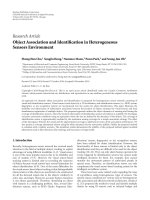
For example, Figure 1 illustrates a transmitter T and a
set of receivers. The grid is partitioned into four quadrants
from the computed receiver centroid. The set of perimeter
receivers, as the farthest receivers from the centroid in each
quadrant (I to IV), form a rudimentary bounding area for
the location of the transmitter. The A
γ
algorithm computes
hyperbolic areas between all pairs of perimeter receivers, in
III
IVIII
1
2

3
4
5
6
7
8
T
R
R
R
R
R
R
R
R
10009008007006005004003002001000
Tr an sm it te r
Centroid
Receiver
Perimeter Rcvr
0
100
200
300
400
500
600
700
800
900

1000
Figure 1: Example of perimeter receivers.
this case between all possible pairs in N ={R
3
, R
4
, R
7
, R
5
}.
Additional receiver pairs are formed between the remaining
nonperimeter receivers
{R
1
, R
2
, R
6
, R
8
} and the perimeter
receivers of other quadrants. Receiver R
6
, for instance, is
situated in quadrant II, so it is included in a receiver pair with
eachperimeterreceiverin
{R
3
, R

7
, R
5
}.
In terms of complexity, the A
γ
algorithm is equivalent to
A
β
.Givenn receivers and four perimeter receivers such that
|N |=4, A
γ
executes in time

4
2

+3(n− 4) = 3n− 6 ≈ O(n).
The candidate area for the location of a malicious
transmitter is computed as the intersection of a set of
hyperbolic areas,
H
α
, H
β
,orH
γ
, determined according to
Algorithms 1, 2,or3.
Definition 3 (candidate area). Let

G be the set of all (x, y)
coordinates in our sample Euclidian space. Let
V ⊆ G be
the subset of all coordinates situated on the road layout
of a vehicular scenario. Then the grid candidate area GA

,
where 
∈{α, β, γ}, is defined as the subset of grid points
in
G situated in the intersection of every hyperbolic area
computed according to Algorithms A
α
, A
β
,orA
γ
:
GA

=
⎧
⎨
⎩
p
k
: p
k
∈ G, p
k

∈
h≤m

h=1
A
h
∈ H

where  ∈

α, β, γ

, m =



H




⎫
⎬
⎭
.
(17)
Similarly, the vehicular candidate area VA

,where ∈
{

α, β, γ}, is defined as the subset of vehicular layout points
in
V situated in the intersection of every hyperbolic area
computed according to Algorithms A
α
, A
β
,orA
γ
:
VA

=
⎧
⎨
⎩
p
k
: p
k
∈ V, p
k
∈
h≤m

h=1
A
h
∈ H


where  ∈

α, β, γ

, m =



H




⎫
⎬
⎭
.
(18)
EURASIP Journal on Wireless Communications and Networking 7
While a candidate area contains a malicious transmitter
with probability C, the tracking of a mobile device requires a
unique point in Euclidian space to be deemed the likeliest
position for the attacker. In free space, we can use the
centroid of a candidate area, which is calculated as the
average of all the (x, y) coordinates in this area. In a vehicular
scenario, we use the road location closest to the candidate
area centroid.
Definition 4 (centroids). The grid centroid of a given GA,
denoted as Gχ, consists of the average (x, y) coordinates of
all points within the GA:

Gχ
=

x
G
, y
G

, such that x
G
=

|GA|
i=1
x
i
|GA|
, y
G
=

|GA|
i=1
y
i
|GA|
,
∀p
i
=


x
i
, y
i

∈
GA.
(19)
The vehicular centroid of a given VA, represented as Vχ, is the
closest vehicular point to the average coordinates of all points
within the VA:
Vχ
= v
k
, such that v
k
∈ V, p
h
=

x
V
, y
V

,
where x
V
=


|VA |
i=1
x
i
|VA |
, y
V
=

|VA |
i=1
y
i
|VA |
,
∀p
i
=

x
i
, y
i

∈ VA ,
δ

p
h

, v
k

≤
δ

p
h
, v
j

, ∀v
j
∈ V.
(20)
4.3. Tracking a Mobile Attacker. We extend HPB to approxi-
mate the path followed by a mobile attacker, as it continues
transmitting. By computing a new candidate area for each
attack message received, a malicious node can be tracked
using a set of consecutive candidate positions and the
direction of travel inferred between these points. We establish
a mobility path in our vehicular scenario as a sequence of
vehicular layout (x, y) coordinates over time, along with a
mobile transmitter’s direction of travel at every point.
Definition 5. A mobility path
P is defined as a set of
consecutive coordinates p
i
= (x
i

, y
i
)andanglesoftravelθ
i
over a time interval T:
P =

p
i
, θ
i

: p
i
=

x
i
, y
i

is the transmitter location
at t
i
∈ T, θ
i
= atan 2

y
i

− y
i−1
, x
i
− x
i−1

,
(21)
where atan 2 is an inverse tangent function returning values
over the range [
−π,+π] to take direction into account (as
first defined for the Fortran 77 programming language [25]).
In order to approximate the dynamically changing
position of an attacker, we discretize the time domain
T into a series of time intervals t
i
. At each discrete t
i
,
we sample a snapshot of the vehicular network topology
consisting of a set of receiving devices and their locations.
Our approach is analogous to the discretization phase in
digital signal processing, where a continuous analog radio
signal is sampled periodically for conversion to digital form.
We thus estimate the mobility path
P taken by an attacker by
executing an HPB algorithm for an attack message received at
every interval t
i

over a time period T. The vehicular centroids
of the resulting candidate areas constitute the estimated
attacker positions, and the angle from one estimated point
to the next determines the approximated direction of
travel.
Algorithm 4 (mobile attacker tracking). Let M be the set of
consecutive attack messages received over a time interval.
Then the estimated mobility path

P
of a transmitter over the
message base M is computed as follows:

P =


p
i
,

θ
i

:

p
i
=



x
i
, y
i

=
Vχ
i
for m
i
∈ M,

θ
i
= atan 2


y
i
− y
i−1
, x
i
− x
i−1


.
(22)
For every attack message m

i
∈ M,anestimated
transmitter location

p
i
must be determined. An execution
of HPB using the RSS values corresponding to m
i
yields a
vehicular candidate area VA
i
,asputforthinDefinition 3.
TheroadcentroidofVA
i
is computed as Vχ
i
, according
to Definition 4. It is by definition the closest point in the
vehicular layout to the averaged center of the VA
i
,and
thus the natural choice for an estimated value

p
i
of the
true transmitter location p
i
. The direction of travel of a

transmitter is stated in Definition 5 as the angle between
consecutive positions in Euclidian space. We follow the same
logic to compute the estimated direction of travel

θ
i
between
transmitted messages m
i−1
and m
i
as the angle between the
corresponding estimated positions

p
i−1
and

p
i
.
Example 1. Figure 2 depicts an example mobility path of a
malicious insider, with consecutive traveled points labeled
from 1 to 20. The transmitter broadcasts an attack message
at every fourth location, labeled as points 4, 8, 12, 16 and 20.
For each attack message, we execute the A
γ
HPB varia-
tion, for confidence level C
= 0.95, using eight randomly

positioned receivers, and a vehicular candidate area VA
γ
is
computed. The estimated locations and directions of travel
are depicted in Figure 3. The initial point’s direction of travel
cannot be estimated, as there is no previous point from
which to ascertain a traveled path. In this example, point 4
is localized at 100 meters from its true position, points 8,
16 and 20 at 25 meters, while point 12 is found in its exact
location.
5. Performance Evaluation
We describe a simulated vehicular scenario to evaluate
the localization and tracking performance of the extended
HPB mechanisms described in Section 4.2.Inorderto
model a mobile attacker transmitting at 2.4 GHz, we employ
Rappaport’s log-normal shadowing model [22] to generate
simulated RSS values at a set of receivers, taking into
account an independently random amount of signal shad-
owing experienced at each receiving device. According to
Rappaport, the log-normal shadowing model has been used
extensively in experimental settings to capture radio signal
8 EURASIP Journal on Wireless Communications and Networking
12345678910
11
12
13
14
15
16
17

18
19
20
600550500450400350300250200
200
250
300
350
400
450
500
550
600
Figure 2: Example of attacker mobility path.
4
8
12
16
20
600550500450400350300250200
200
250
300
350
400
450
500
550
600
Figure 3: Example of mobile attacker localization.

propagation characteristics, in both indoor and outdoor
channels, including in mobility scenarios. In our previous
work, we have evaluated HPB results with both log-normal
shadowing simulated RSS values and RSS reports harvested
from an outdoor field experiment at 2.4 GHz [9]. We found
that the simulated and experimental location estimation
results are nearly identical, indicating that at this frequency,
the log-normal shadowing model is an appropriate tool for
generating realistic RSS values.
We compare the success rates of the A
α
, A
β
and A
γ
algorithms at estimating a malicious transmitter’s location
within a candidate area, as well as the relative sizes of the
grid and vehicular candidate areas. We model a mobile
transmitter’s path through a vehicular scenario and assess the
success in tracking it by measuring the distance between the
actual and estimated positions, in addition to the difference
between the approximated direction of travel and the real
one.
5.1. Hyperbolic Position Bounding of Vehicular Devices. Our
simulation uses a one square kilometer urban grid, as
depicted in Figure 4. We evaluate the all-pairs A
α
, 4-pair
Nixon Farm Dr.
Perth St. Perth St.

Huntley Rd.
N
Fowler St.
McBean St.
Martin St.
Figure 4: Urban scenario—Richmond, Ontario.
set A
β
and perimeter-pairs A
γ
HPB algorithms with four,
eight, 16 and 32 receivers. In each HPB execution, four
of the receivers are fixed road-side units (RSUs) stationed
at intersections. The remaining receivers are randomly
positioned on-board units (OBUs), distributed uniformly on
the grid streets. Every HPB execution also sees a transmitter
placed at a random road position within the inner square of
the simulation grid. We assume that in a sufficiently dense
urban setting, RSUs are positioned at most intersections. As a
result, any transmitter location is geographically surrounded
by four RSUs within radio range. For each defined number of
receivers and two separate confidence levels C
∈{0.95, 0.90},
the HPB algorithms, A
α
, A
β
and A
γ
, are executed 1000

times. For every execution, RSS values are generated for
each receiver from the log-normal shadowing model. We
adopt existing experimental path loss parameter values from
large-scale measurements gathered at 2.4 GHz by Liechty
et al. [26, 27]. From η
= 2.76 and a signal shadowing
standard deviation σ
= 5.62, we augment the simulated RSS
values with an independently generated amount of random
shadowing to every receiver in a given HPB execution. Since
the EIRP used by a malicious transmitter is unknown, a
probable range is computed according to Heuristic 1.
For every HPB execution, whether the A
α
, A
β
or A
γ
algorithm is used, we gather three metrics: the success rate
in localizing the transmitter within a computed candidate
area GA; the size of the unconstrained candidate area GA
as a percentage of the one square kilometer grid; the size of
the candidate area restricted to the vehicular layout VA as a
percentage of the grid. The success rate and candidate area
size results we obtain are deemed 90% accurate within a 2%
and 0.8% confidence interval, respectively. The average HPB
execution times for each algorithm on an HP Pavilion laptop
with an AMD Turion 64
× 2 dual-core processor are shown
in Ta bl e 1 . As expected from our complexity analysis, the A

α
EURASIP Journal on Wireless Communications and Networking 9
321684
Number of receivers
A
γ
A
β
A
α
0
10
20
30
40
50
60
70
80
90
100
Success rate
Figure 5: Success rate for C = 0.95.
Table 1: Average HPB execution time (seconds).
#Rcvrs A
γ
A
β
A
α

Mean Std dev. Mean Std dev. Mean Std dev.
4 0.005 0.000 0.023 0.001 0.023 0.001
8 0.023 0.001 0.045 0.001 0.104 0.003
16 0.075 0.001 0.090 0.002 0.486 0.142
32 0.215 0.059 0.195 0.053 2.230 0.766
variation is markedly slower, and the computational costs
increase as additional receivers participate in the location
estimation effort. For example in the case of eight receivers,
a single execution of A
γ
takes 23 milliseconds, while A
α
requires over 100 milliseconds.
The comparative success rates of the A
α
, A
β
and A
γ
approaches are illustrated in Figure 5, for confidence level
C
= 0.95. While A
γ
exhibits the best localization success
rate, every algorithm sees its performance degrade as more
receivers are included. With four receivers for example, all
three variations successfully localize a transmitter 94-95% of
the time. However with 32 receivers, A
γ
succeeds in 79%

of the cases, while A
β
and A
α
do so in 71% and 50% of
executions. Given that each receiver pair takes into account
an amount of signal shadowing based on the confidence level
C, it also probabilistically ignores a portion (1
− C)ofthe
shadowing.Asmorereceiversandthusmorereceiverpairs
are added, the error due to excluded shadowing accumulates.
The results obtained for confidence level C
= 0.90 follow the
same trend, although the success rates are slightly lower.
Figures 6 and 7 show the grid and vehicular candi-
date area sizes associated with our simulation scenario, as
computed with algorithms A
α
, A
β
and A
γ
, for confidence
level C
= 0.95. The size of the grid candidate area GA
corresponds to 21% of the simulation grid, with four
receivers, for both A
β
and A
α

, while A
γ
narrows the area
to only 7%. In fact, the A
γ
approach exhibits a GA size
that is independent of the number of receivers. Yet for A
β
and A
α
, the GA size is noticeably lower with additional
receivers. This finding reflects the use of perimeter receivers
with A
γ
. These specialized receivers serve to restrict the GA
to a particular portion of the simulation grid, even with
few receivers. However, this variation does not fully exploit
the presence of additional receiving devices, as these only
support the GA determined by the perimeter receivers. The
size of the vehicular candidate area VA follows the same
trend, with a near constant size of 0.64% to 1% of the grid for
A
γ
, corresponding to a localization granularity within an area
less than 100 m
× 100 m, assuming the transmitter is aboard
a vehicle traveling on a road. The A
β
and A
α

algorithms
compute vehicular candidate area sizes that decrease as more
receivers are taken into account, with A
α
yielding the best
localization granularity. But even with four receivers, A
β
and
A
α
localize a transmitter within a vehicular layout area of
1.6% of the grid, or 125 m
× 125 m.
Generally, both the GA and VA sizes decrease as the
number of receivers increases, since additional hyperbolic
areas pose a higher number of constraints on a candidate
area,thusdecreasingitsextent.WeseeinFigures6 and 7 that
A
β
consistently yields larger candidate areas than A
α
for the
same reason, as A
α
generates a significantly greater number
of hyperbolic areas. For example, while A
α
computes an
average GA
α

of 10% and 3% of the simulation grid with eight
and 16 receivers, A
β
yields areas of 15% and 9%, respectively.
By contrast, A
γ
yields a GA size of 5-6% but its reliability is
greater, as demonstrated by the higher success rates achieved.
The nearly constant 5% GA size computed with A
γ
has an
average success rate of 81% for 16 receivers, while the 9% GA
generated by A
β
is 79% reliable and the 3% GA obtained with
A
α
features a dismal 68% success rate. Indeed, Figures 5 and 6
taken together indicate that smaller candidate areas provide
increased granularity at the cost of lower success rates, and
thus decreased reliability. This phenomenon is consistent
with the intuitive expectation that a smaller area is less likely
to contain the transmitter.
5.2. Tracking a Vehicular Device. We generate 1000 attacker
mobility paths
P, as stipulated in Definition 5, of 20 consecu-
tive points evenly spaced at every 25 meters. Each path begins
at a random start location along the central square of the
simulation grid depicted in Figure 4. We keep the simulated
transmitter location within the area covered by four fixed

RSUs, presuming that an infinite grid features at least four
RSUs within radio range of a transmitter. The direction of
travel for the start location is determined randomly. Each
subsequent point in the mobile path is contiguous to the
previous point, along the direction of travel. Upon reaching
an intersection in the simulation grid, a direction of travel is
chosen randomly among the ones available from the current
position, excluding the reverse direction.
The A
α
, A
β
and A
γ
algorithms are executed at every
fourth point p
i
of each mobility path P, corresponding to a
transmitted attack signal at every 100 meters. The algorithms
10 EURASIP Journal on Wireless Communications and Networking
35302520151050
Number of receivers
GA
γ
GA
β
GA
α
0
5

10
15
20
25
Candidate area size (%)
Figure 6: Grid candidate area size for C = 0.95.
35302520151050
Number of receivers
VA
γ
VA
β
VA
α
0
0.2
0.4
0.6
0.8
1
1.2
1.4
1.6
1.8
Candidate area size (%)
Figure 7: Vehicular candidate area size for C = 0.95.
are executed for confidence levels C ∈{0.95,0.90},with
each of four, eight, 16 and 32 receivers. In every case, the
receivers consist of four static RSUs, and the remaining are
OBUs randomly placed at any point on the simulated roads.

For each execution of A
α
, A
β
and A
γ
,avehicular
candidate area VA is computed, and its centroid Vχ is taken
as the probable location of the transmitter, as described in
Algorithm 4. Two metrics are aggregated over the executions:
the root mean square location error, as the distance in meters
between the actual transmitter location p
i
and its estimated
position

p
i
= Vχ
i
; and the root mean square angle error
between the angle of travel θ
i
for each consecutive actual
321684
Number of receivers
A
γ
A
β

A
α
0
20
40
60
80
100
120
140
Location error (meters)
Figure 8: Location error for C = 0.95.
transmitter location and the angle

θ
i
computed for the
approximated locations.
The location error for the A
α
, A
β
and A
γ
algorithms,
given confidence level C
= 0.95, is illustrated in Figure 8.
As expected, the smaller VA sizes achieved with a greater
number of receivers for A
α

and A
β
correspond to a more
precise transmitter localization. The location error associated
with the A
α
algorithm is smaller, compared to A
β
, for the
same reason. Correspondingly, the nearly constant VA size
obtained with A
γ
yields a similar result for the location error.
For instance with confidence level C
= 0.95, eight and 16
receivers produce a location error of 114 and 79 meters,
respectively, with A
α
but of 121 and 102 meters with A
β
.The
location error with A
γ
is once more nearly constant, at 96
and 91 meters. The use of all receiver pairs to compute a VA
with A
α
allows for localization that is up to 40–50% more
precise than grouping the receivers in sets of four or relying
on perimeter receivers when 16 or 32 receiving devices are

present. Despite its granular localization performance, the
A
α
approach works best with large numbers of receivers,
which may not consistently be realistic in a practical setting.
Another important disadvantage of the A
α
approach lies in
its large complexity of O(n
2
)forn receivers, when compared
to A
β
and A
γ
with a complexity of O(n), as discussed in
Section 4.2.
Figure 9 plots the root mean square location error in
terms of VA size for the three algorithms. While A
α
and
A
β
yield smaller VAs for a large number of receivers, the
VAs computed with A
γ
offer more precise localization with
respect to their size. For example, a 0.7% VA size obtained
with A
γ

features a 96 meter location error, while a similar
size VA computed with A
β
and A
α
generates a 102 and 114
meter location error, respectively.
The error in estimating the direction of travel exhibits
little variation in terms of number of receivers and choice
EURASIP Journal on Wireless Communications and Networking 11
1.61.41.210.80.60.40.20
Vehicular candidate area size (%)
VA
γ
VA
β
VA
α
40
50
60
70
80
90
100
110
120
130
140
Location error (meters)

Figure 9: Location error for vehicular candidate area size.
321684
Number of receivers
A
γ
A
β
A
α
0
10
20
30
40
50
60
70
80
Angle error (degrees)
Figure 10: Direction of travel angle error for C = 0.95.
of HPB algorithm, as shown in Figure 10. With eight and 16
receivers, for confidence level C
= 0.95, A
β
approximates
the angle of travel between two consecutive points within
77
◦
and 71
◦

, respectively, whereas A
α
estimates it within 76
◦
and 63
◦
. A
γ
exhibits a slightly higher direction error at 76
◦
and 77
◦
. It should be noted that for all three algorithms,
for all numbers of receivers, the range of angle errors
only spans 14
◦
. So while the granularity of localization
is contingent upon the HPB methodology used and the
number of receivers, the three variations perform similarly
in estimating the general direction of travel.
6. Discussion
The location error results of Figure 8 shed an interesting
light on the HPB success rates discussed in Section 5.1.For
example in the presence of 32 receivers, for confidence level
C
= 0.95, only 50% of A
α
executions yield a candidate area
containing a malicious transmitter, as shown in Figure 5.
Yet the same scenario localizes a transmitter with a root

mean square location error of 45 meters of its true location,
whether it lies within the corresponding candidate area
or not. This indicates that while a candidate area may be
computed in the wrong position, it is in fact rarely far from
the correct transmitter location. This may be a result of
our strict definition of a successful execution, where only
a candidate area in the intersection of all hyperbolic areas
is considered. We have observed in our simulations that a
candidate area may be erroneous solely because of a single
misplaced hyperbolic area, which results in either a wrong
location or an empty candidate area. In our simulations
tracking a mobile attacker, we notice that while A
γ
and A
β
generate an empty VA for 10% and 14% of executions, A
α
does so in 31% of the cases. This phenomenon is likely
due to the greater number of hyperbolic areas generated
with the A
α
approach and the subsequent greater likelihood
of erroneously situated hyperbolic areas. While the success
rates depicted in Figure 5 omit the executions yielding
empty candidate areas as inconclusive, future work includes
devising a heuristic to recompute a set of hyperbolic areas in
the case where their common intersection is empty.
In comparing the location accuracy of HPB with related
technologies, we find that, for example, differential GPS
devices can achieve less than 10 meter accuracy. However,

this technology is better suited to self-localization efforts
relying on a device’s assistance and cannot be depended upon
for the position estimation of a noncooperative adversary.
The FCC has set forth regulations for the network-based
localization of wireless handsets in emergency 911 call
situations. Service providers are expected to locate a calling
device within 100 meters 67% of the time and within 300
meters in 95% of cases [28]. In the minimalist case involving
four receivers, the HPB perimeter-pairs variation A
γ
localizes
a transmitting device with a root mean square location error
of 107 meters. This translates into a location accuracy of
210 meters in 95% of cases and of 104 meters in 67%
of executions. While the former case is fully within FCC
guidelines, the latter is very close. With a larger number
of receivers, for example, eight receiving devices, A
γ
yields
an accuracy of 188 meters 95% of the time and of 93
meters in 67% of cases. Although HPB is designed for the
location estimation of a malicious insider, its use may be
extended to additional applications such as 911 call origin
localization, given that its performance closely matches the
FCC requirements for emergency services.
7. Concl usion
We extend a hyperbolic position bounding (HPB) mecha-
nism to localize the originator of an attack signal within
a vehicular network. Because of our novel assumption that
12 EURASIP Journal on Wireless Communications and Networking

the message EIRP is unknown, the HPB location estimation
approach is suitable to security scenarios involving malicious
or uncooperative devices, including insider attacks. Any
countermeasure to this type of exploit must feature minimal-
ist assumptions regarding the type of radio equipment used
by an attacker and expect no cooperation with localization
efforts on the part of a perpetrator.
We devise two additional HPB-based approaches to com-
pute hyperbolic areas between pairs of trusted receivers by
grouping them in sets and establishing perimeter receivers.
We demonstrate that due to the dynamic computation of
a probable EIRP range utilized by an attacker, our HPB
algorithms are impervious to varying power attacks. We
extend the HPB algorithms to track the location of a mobile
attacker transmitting along a traveled path.
The performance of all three HPB variations is evaluated
in a vehicular scenario. We find that the grouped receivers
method yields a localization success rate up to 11% higher
for a 6% increase in candidate area size over the all-
pairs approach. We also observe that the perimeter-pairs
algorithm provides a more constant candidate area size,
independently of the number of receivers, for a success rate
up to 13% higher for a 2% increase in candidate area size
over the all-pairs variation. We conclude that the original
HPB mechanism using all pairs of receivers produces a
smaller localization error than the other two approaches,
when a large number of receiving devices are available.
We observe that for a confidence level of 95%, the former
approach localizes a mobile transmitter with a granularity
as low as 45 meters, up to 40–50% more precisely than the

grouped receivers and perimeter-pairs methods. However,
the computational complexity of the all-pairs variation is
significantly greater, and its performance with fewer receivers
is less granular than the perimeter-pairs method. Of the
two approaches with complexity O(n), the perimeter-pairs
method yields a success rate up to 8% higher for consistently
smaller candidate area sizes, location, and direction errors.
In a vehicular scenario, we achieve a root mean square
location error of 107 meters with four receivers and of
96 meters with eight receiving devices. This granularity is
sufficient to satisfy the FCC-mandated location accuracy
regulations for emergency 911 services. Our HPB mechanism
may therefore be adaptable to a wide range of applications
involving network-based device localization assuming nei-
ther target node cooperation nor knowledge of the EIRP.
We have demonstrated the suitability of the hyperbolic
position bounding mechanism for estimating the candidate
location of a vehicular network malicious insider and for
tracking such a device as it moves throughout the network.
Future research is required to assess the applicability of the
HPB localization and tracking mechanisms in additional
types of wireless and mobile technologies, including wireless
access networks such as WiMAX/802.16.
Acknowledgments
The authors gratefully acknowledge the financial support
received for this research from the Natural Sciences and
Engineering Research Council of Canada (NSERC) and the
Automobile of the 21st Century (AUTO21) Network of
Centers of Excellence (NCE).
References

[1] IEEE Intelligent Transportation Systems Committee, “IEEE
Trial-Use Standard for Wireless Access in Vehicular
Environments—Security Services for Applications and
Management Messages,” IEEE Std 1609.2-2006, July 2006.
[2] R. Anderson, M. Bond, J. Clulow, and S. Skorobogatov, “Cryp-
tographic processors—a survey,” Proceedings of the IEEE, vol.
94, no. 2, pp. 357–369, 2006.
[3] R. Anderson and M. Kuhn, “Tamper resistance: a cautionary
note,” in Proceedings of the 2nd USENIX Wor kshop on Elec-
tronic Commerce, pp. 1–11, Oakland, Calif, USA, November
1996.
[4] National Institute of Standards and Technology, “Security
Requirements for Cryptographic Modules,” Federal Informa-
tion Processing Standards 140-2, NIST, May 2001.
[5] IBM, “IBM 4764 PCI-X Cryptographic Coprocessor,”
.
[6] D. E. Williams, “A Concept for Universal Identification,” White
paper, SANS Institute, December 2001.
[7] SeVeCom, “Security architecture and mechanisms for
V2V/V2I, deliverable 2.1,” Tech. Rep. D2.1, Secure Vehicle
Communication, Paris, France, August 2007, edited by
Antonio Kung.
[8] C. Laurendeau and M. Barbeau, “Insider attack attribution
using signal strength-based hyperbolic location estimation,”
Security and Communication Networks, vol. 1, no. 4, pp. 337–
349, 2008.
[9] C. Laurendeau and M. Barbeau, “Hyperbolic location esti-
mation of malicious nodes in mobile WiFi/802.11 networks,”
in Proceedings of the 2nd IEEE LCN Workshop on User
MObility and VEhicular Networks (ON-MOVE ’08), pp. 600–

607, Montreal, Canada, October 2008.
[10] A. Boukerche, H. A. B. F. Oliveira, E. F. Nakamura, and A. A.
F. Loureiro, “Vehicular ad hoc networks: a new challenge for
localization-based systems,” Computer Communications, vol.
31, no. 12, pp. 2838–2849, 2008.
[11] R. Parker and S. Valaee, “Vehicular node localization
using received-signal-strength indicator,” IEEE Transactions on
Vehicular Technology, vol. 56, no. 6, part 1, pp. 3371–3380,
2007.
[12] J P. Hubaux, S.
ˇ
Capkun, and J. Luo, “The security and privacy
of smart vehicles,” IEEE Security & Privacy,vol.2,no.3,pp.
49–55, 2004.
[13] S.
ˇ
Capkun and J P. Hubaux, “Secure positioning in wireless
networks,” IEEE Journal on Selected Areas in Communications,
vol. 24, no. 2, pp. 221–232, 2006.
[14] S. Brands and D. Chaum, “Distance-bounding protocols,” in
Proceedings of the Workshop on the Theory and Application of
Cryptographic Techniques on Advances in Cryptology (EURO-
CRYPT ’94), vol. 765 of Lecture Notes in Computer Sc ience,pp.
344–359, Springer, Perugia, Italy, May 1994.
[15] B. Xiao, B. Yu, and C. Gao, “Detection and localization of
sybil nodes in VANETs,” in Proceedings of the Workshop on
Dependability Issues in Wireless Ad Hoc Networks and Sensor
Networks (DIWANS ’06),pp.1–8,LosAngeles,Calif,USA,
September 2006.
EURASIP Journal on Wireless Communications and Networking 13

[16] T. Leinm
¨
uller, E. Schoch, and F. Kargl, “Position verification
approaches for vehicular ad hoc networks,” IEEE Wireless
Communications, vol. 13, no. 5, pp. 16–21, 2006.
[17] J. R. Douceur, “The Sybil attack,” in Peer-to-Peer Systems,
vol. 2429 of Lecture Notes in Computer Science, pp. 251–260,
Springer, Berlin, Germany, 2002.
[18] L. Tang, X. Hong, and P. G. Bradford, “Privacy-preserving
secure relative localization in vehicular networks,” Security and
Communication Networks, vol. 1, no. 3, pp. 195–204, 2008.
[19] G. Yan, S. Olariu, and M. C. Weigle, “Providing VANET
security through active position detection,” Computer Com-
munications, vol. 31, no. 12, pp. 2883–2897, 2008.
[20] N. Mirmotahhary, A. Kohansal, H. Zamiri-Jafarian, and
M. Mirsalehi, “Discrete mobile user tracking algorithm via
velocity estimation for microcellular urban environment,” in
Proceedings of the 67th IEEE Vehicular Technology Conference
(VTC ’08), pp. 2631–2635, Singapore, May 2008.
[21] Z. R. Zaidi and B. L. Mark, “Real-time mobility tracking
algorithms for cellular networks based on Kalman filtering,”
IEEE Transactions on Mobile Computing, vol. 4, no. 2, pp. 195–
208, 2005.
[22] T. S. Rappaport, Wireless Communications: Principles and
Practice, Prentice-Hall, Upper Saddle River, NJ, USA, 2nd
edition, 2002.
[23] C. Laurendeau and M. Barbeau, “Probabilistic evidence
aggregation for malicious node position bounding in wireless
networks,” Journal of Networks, vol. 4, no. 1, pp. 9–18, 2009.
[24] Y. Chen, K. Kleisouris, X. Li, W. Trappe, and R. P. Martin,

“The robustness of localization algorithms to signal strength
attacks: a comparative study,” in Proceedings of the 2nd IEEE
International Conference on Distributed Computing in Sensor
Systems (DCOSS ’06), vol. 4026 of Lecture Notes in Computer
Science, pp. 546–563, Springer, San Francisco, Calif, USA, June
2006.
[25] American National Standards Institute, “Programming Lan-
guage FORTRAN,” ANSI Standard X3.9-1978, 1978.
[26] L. C. Liechty, Path loss measurements and model analysis of
a 2.4 GHz w ireless network in an outdoor environment ,M.S.
thesis, Georgia Institute of Technology, Atlanta, Ga, USA,
August 2007.
[27] L. C. Liechty, E. Reifsnider, and G. Durgin, “Developing
the best 2.4 GHz propagation model from active network
measurements,” in Proceedings of the 66th IEEE Vehicular
Technology Conference (VTC ’07), pp. 894–896, Baltimore, Md,
USA, September-October 2007.
[28] Federal Communications Commission, 911 Service, FCC
Code of Federal Regulations, Title 47, Part 20, Section 20.18,
October 2007.