Báo cáo hóa học: " Recursive Principal Components Analysis Using Eigenvector Matrix Perturbation" docx
Bạn đang xem bản rút gọn của tài liệu. Xem và tải ngay bản đầy đủ của tài liệu tại đây (820.41 KB, 8 trang )
EURASIP Journal on Applied Signal Processing 2004:13, 2034–2041
c
2004 Hindawi Publishing Corporation
Recursive Principal Components Analysis
Using Eigenvector Matrix Perturbation
Deniz Erdogmus
Department of Computer Science and Engineering, CSE, Oregon Graduate Institute, Oregon Health & Science University,
Beaverton, OR 97006, USA
Email:
Yadunandana N. Rao
Computational NeuroEngineering Laboratory (CNEL), Department of Electrical & Computer Engineering (ECE),
University of Florida, Gainesville, FL 32611, USA
Email: fl.edu
Hemanth Peddaneni
Computational NeuroEngineering Laboratory (CNEL), Department of Electrical & Computer Engineering (ECE),
University of Florida, Gainesville, FL 32611, USA
Email: fl.edu
Anant Hegde
Computational NeuroEngineering Laboratory (CNEL), Department of Electrical & Computer Engineering (ECE),
University of Florida, Gainesville, FL 32611, USA
Email: fl.edu
Jose C. Principe
Computational NeuroEngineering Laboratory (CNEL), Department of Electrical & Computer Engineering (ECE),
University of Florida, Gainesville, FL 32611, USA
Email: fl.edu
Received 4 December 2003; Revised 19 March 2004; Recommended for Publication by John Sorensen
Principal components analysis is an important and well-studied subject in statistics and signal processing. The literature has an
abundance of algorithms for solving this problem, where most of these algorithms could be grouped into one of the following
three approaches: adaptation based on Hebbian updates and deflation, optimization of a second-order statistical criterion (like
reconstruction error or output variance), and fixed point update rules with deflation. In this paper, we take a completely differ-
ent approach that avoids deflation and the optimization of a cost function using gradients. The proposed method updates the
eigenvector and eigenvalue matrices simultaneously with every new sample such that the estimates approximately track their true
values as would be calculated from the current sample estimate of the data covariance matrix. The performance of this algorithm is
compared with that of traditional methods like Sanger’s rule and APEX, as well as a structurally similar matr ix perturbation-based
method.
Keywords and phrases: PCA, recursive a lgorithm, rank-one matrix update.
1. INTRODUCTION
Principal components analysis (PCA) is a well-known statis-
tical technique that has been widely applied to solve impor-
tant signal processing problems like feature extract ion, sig-
nal estimation, detection, and speech separation [1, 2, 3, 4].
Many analytical techniques exist, wh ich can solve PCA once
the entire input data is known [5]. However, most of the
analytical methods require extensive matrix operations and
hence they are unsuited for real-time applications. Further,
in many applications such as direction of arrival (DOA)
tracking, adaptive subspace estimation, and so forth, signal
statistics change over time rendering the block methods vir-
tually unacceptable. In such cases, fast, adaptive, on-line so-
lutions are desirable. Majority of the existing algorithms for
PCA are based on standard gradient procedures [2, 3, 6, 7,
8, 9], which are extremely slow converging, and their perfor-
mance depends heavily on step-sizes used. To alleviate this,
Recursive Principal Components Analysis 2035
subspace methods have been explored [10, 11, 12]. How-
ever, many of these subspace techniques are computation-
ally intensive. The recently proposed fixed-point PCA algo-
rithm [13] showed fast convergence with little or no change
in complexity compared with gradient methods. However,
this method and most of the existing methods in literature
rely on using the standard deflation technique, which brings
in sequential convergence of principal components that po-
tentially reduces the overall speed of convergence. We re-
cently explored a simultaneous principal component extrac-
tion algorithm called SIPEX [14] which reduced the gradient
search only to the space of orthonormal matrices by using
Givens rotations. Althoug h SIPEX resulted in fast and simul-
taneous convergence of all principal components, the algo-
rithm suffered from high computational complexity due to
the involved trigonometric function evaluations. A recently
proposed alternative approach suggested iterating the eigen-
vector estimates using a first-order matrix perturbation for-
malism for the sample covariance estimate with every new
sample obtained in real time [15]. However, the performance
(speed and accuracy) of this algorithm is hindered by the
general Toeplitz structure of the perturbed covariance ma-
trix. In this paper, we will present an algorithm that under-
takes a similar perturbation approach, but in contrast, the
covariance matrix will be decomposed into its eigenvectors
and eigenvalues at all times, which will reduce the pertur-
bation step to be employed on the diagonal eigenvalue ma-
trix. This further restriction of structure, as expected, allevi-
ates the difficulties encountered in the operation of the pre-
vious first-order perturbation algorithm, resulting in a fast
converging and accurate subspace tracking algorithm.
This paper is organized as follows. First, we present a
brief definition of the PCA problem to have a self-contained
paper. Second, the proposed recursive PCA (RPCA) algo-
rithm is motivated, derived, and extended to non-stationary
and complex-valued signal situations. Next, a set of com-
puter experiments is presented to demonstrate the conver-
gence speed and accuracy characteristics of RPCA. Finally,
we conclude the paper with remarks and observations about
the algorithm.
2. PROBLEM DEFINITION
PCA is a well-known problem and is extensively studied in
the literature as we have pointed out in the introduction.
However, for the sake of completeness, we will provide a brief
definition of the problem in this s ection. For simplicity, and
without loss of generality, we will consider a real-valued zero-
mean, n-dimensional random vector x and its n projections
y
1
, , y
n
such that y
j
= w
T
j
x,wherew
j
’s are unit-norm vec-
tors defining the projection dimensions in the n-dimensional
input space.
The first principal component direction is defined as the
solution to the following constrained optimization problem,
where R is the input covariance matrix:
w
1
= arg max
w
w
T
Rw subject to w
T
w = 1. (1)
The subsequent principal components are defined by includ-
ing additional constraints to the problem that enforce the or-
thogonality of the sought component to the previously dis-
covered ones:
w
j
= arg max
w
w
T
Rw,s.t.w
T
w = 1, w
T
w
l
= 0, l<j. (2)
The overall solution to this problem turns out to be
the eigenvector matrix of the input covariance R.Inpar-
ticular, the principal component directions are given by the
eigenvectors of R arranged according to their corresponding
eigenvalues (largest to smallest) [5].
In signal processing applications, the needs are differ-
ent. The input samples are usually acquired one at a time
(i.e., sequentially as opposed to in batches), which necessi-
tates sample-by-sample update rules for the covariance and
its eigenvector estimates. In this setting, this analytical solu-
tion is of little use, since it is not practical to update the in-
put covariance estimate and solve a full eigendecomposition
problem per sample. However, utilizing the recursive struc-
ture of the covariance estimate, it is possible to come up with
a recursive formula for the eigenvectors of the covariance as
well. This will be described in the next sect ion.
3. RECURSIVE PCA DESCRIPTION
Suppose a sequence of n-dimensional zero-mean wide-sense
stationary input vectors x
k
are arriving, where k is the sample
(time) index. The sample covariance estimate at time k for
the input vector is
1
R
k
=
1
k
k
i=1
x
i
x
T
i
=
(k − 1)
k
R
k−1
+
1
k
x
k
x
T
k
. (3)
Let R
k
= Q
k
Λ
k
Q
T
k
and R
k−1
= Q
k−1
Λ
k−1
Q
T
k−1
,whereQ and
Λ denote the orthonormal eigenvector and diagonal eigen-
value matrices, respectively. Also define α
k
= Q
T
k−1
x
k
.Substi-
tuting these definitions in (3), we obtain the following recur-
sive formula for the eigenvectors and eigenvalues:
Q
k
kΛ
k
Q
T
k
= Q
k−1
(k − 1)Λ
k−1
+ α
k
α
T
k
Q
T
k−1
. (4)
Clearly, if we can determine the eigendecomposition of the
matrix [(k − 1)Λ
k−1
+ α
k
α
T
k
], which is denoted by V
k
D
k
V
T
k
,
where V is orthonormal and D is diagonal, then (4)becomes
Q
k
kΛ
k
Q
T
k
= Q
k−1
V
k
D
k
V
T
k
Q
T
k−1
. (5)
1
In practice, if the samples are not generated by a zero-mean process, a
running sample mean estimator could be employed to compensate for this
fact. Then this biased estimator can be replaced by the unbiased version and
the following derivations can be modified accordingly.
2036 EURASIP Journal on Applied Signal Processing
By direct comparison, the recursive update rules for the
eigenvectors and the eigenvalues are determined to be
Q
k
= Q
k−1
V
k
,
Λ
k
=
D
k
k
.
(6)
In spite of the fact that the matrix [(k − 1)Λ
k−1
+ α
k
α
T
k
]hasa
special structure much simpler than that of a general covari-
ance matrix, determining the eigendecomposition V
k
D
k
V
T
k
analytically is difficult. However, especially if k is large, the
problem can be solved in a simpler way using a matrix per-
turbation analysis approach. This will be described next.
3.1. Perturbation analysis for rank-one update
When k is large, the matrix [(k − 1)Λ
k−1
+ α
k
α
T
k
]isstrongly
diagonally dominant; hence (due to the Gershgorin theorem)
its eigenvalues will be close to those of the diagonal portion
(k − 1)Λ
k−1
. In addition, its eigenvectors will also be close to
identity (i.e., the eigenvectors of the diagonal portion of the
sum).
In summary, the problem reduces to finding the eigen-
decomposition of a matrix in the form (Λ + αα
T
), that is, a
rank-one update on a diagonal matrix Λ, using the following
approximations: D = Λ + P
Λ
and V = I + P
V
,whereP
Λ
and
P
V
are small perturbation matrices. The eigenvalue perturba-
tion matr ix P
Λ
is naturally diagonal. With these definitions,
when VDV
T
is expanded, we get
VDV
T
=
I + P
V
Λ + P
Λ
I + P
V
T
= Λ + ΛP
T
V
+ P
Λ
+ P
Λ
P
T
V
+ P
V
Λ
+ P
V
ΛP
T
V
+ P
V
P
Λ
+ P
V
P
Λ
P
T
V
= Λ + P
Λ
+ DP
T
V
+ P
V
D
+ P
V
ΛP
T
V
+ P
V
P
Λ
P
T
V
.
(7)
Equating (7)toΛ+αα
T
, and assuming that the terms P
V
ΛP
T
V
and P
V
P
Λ
P
T
V
are negligible, we get
αα
T
= P
Λ
+ DP
T
V
+ P
V
D. (8)
The orthonormality of V brings an additional equation that
characterizes P
V
. Substituting V = I + P
V
in VV
T
= I,and
assuming that P
V
P
T
V
≈ 0,wehaveP
V
=−P
T
V
.
Combining the fact that the eigenvector perturbation
matrix P
V
is antisymmetric with the fact that P
Λ
and D
are diagonal, the solutions for the perturbation matrices are
found from (8) as follows: the ith diagonal entry of P
Λ
is α
2
i
and the (i, j)th entry of P
V
is α
i
α
j
/(λ
j
+ α
2
j
− λ
i
− α
2
i
)if j = i,
and 0 if j = i.
3.2. The recursive PCA algorithm
The RPCA algorithm is summarized in Algorithm 1.There
are a few practical issues regarding the operation of the algo-
rithm, which will be addressed in this subsection.
(1) Initialize Q
0
and Λ
0
.
(2) At each time instant k do the following.
(a) Get input sample x
k
.
(b) S et memory depth parameter λ
k
.
(c) Calculate α
k
= Q
T
k
−1
x
k
.
(d) Find perturbations P
V
and P
Λ
corresponding
to
1 − λ
k
Λ
k−1
+ λ
k
α
k
α
T
k
.
(e) Update eigenvector and eigenvalue matrices:
Q
k
= Q
k−1
I + P
V
Λ
k
=
1 − λ
k
Λ
k−1
+ P
Λ
.
(f) Normalize the norms of eigenvector estimates
by Q
k
=
Q
k
T
k
,whereT
k
is a diagonal matrix
containing the inverses of the norms of each
column of
Q
k
.
(g) Correct eigenvalue estimates by Λ
k
=
Λ
k
T
−2
k
,
where T
−2
k
is a diagonal matrix containing the
squared norms of the columns of
Q
k
.
Algorithm 1: The recursive PCA algorithm outline.
Selecting the memory depth parameter
In a stationary situation, where we would like to weight
each individual sample equally, this parameter must be set to
λ
k
= 1/k. In this c ase, the recursive update for the covariance
matrix is as shown in (3). In a nonstationary environment, a
first-order dynamical forgetting strategy could be employed
by selecting a fixed decay r ate. Setting λ
k
= λ corresponds to
the following recursive covariance update equation:
R
k
= (1 − λ)R
k
+ λx
k
x
T
k
. (9)
Typically, in this forgetting scheme, λ ∈ (0, 1) is selected to
be very small. Considering that the average memory depth of
this recursion is 1/λ samples, the select ion of this parameter
presents a trade-off between tracking capability and estima-
tion variance.
Initializing the eigenvectors and the eigenvalues
The natural way to initialize the eigenvector matrix Q
0
and
the eigenvalue matrix Λ
0
is to use the first N
0
samples to ob-
tain an unbiased estimate of the covariance matrix and de-
termine its eigendecomposition (N
0
>n).Theiterationsin
step (2) can then be applied to the following samples. This
means in step (2) k = N
0
+1, , N. In the stationary case
(λ
k
= 1/k), this means in the first few iterations of step (2)
the perturbation approximations will be least accurate (com-
pared to the subsequent iterations). This is simply due to
(1 − λ
k
)Λ
k−1
+ λ
k
α
k
α
T
k
not being strongly diagonally dom-
inant for small values of k. Compensating the errors induced
in the estimations at this stage might require a large number
of samples later on.
This problem could be avoided if in the iteration stage
(step (2)) the index k could be started from a large initial
value. In order to achieve this without introducing any bias
Recursive Principal Components Analysis 2037
to the estimates, one needs to use a large number of sam-
ples in the initialization (i.e., choose a large N
0
). In prac-
tice, however, this is undesirable. The alternative is to per-
form the initialization still using a small number of samples
(i.e., a small N
0
), but setting the memory depth parameter to
λ
k
= 1/(k +(τ − 1)N
0
). This way, when the iterations start
at sample k = N
0
+ 1, the algorithm thinks that the initializa-
tion is actually per formed using γ = τN
0
samples. Therefore,
from the point of view of the algorithm, the data set looks
like
x
1
, , x
N
0
, ,
x
1
, , x
N
0
repeated τ times
,
x
N
0
+1
, , x
N
. (10)
The corresponding covariance estimator is then naturally bi-
ased. At the end of the iterations, the estimated covariance
matrix is
R
N,biased
=
N
N +(τ − 1)N
0
R
N
+
(τ − 1)N
0
N +(τ − 1)N
0
R
N
0
, (11)
where R
M
= (1/M)
M
j=1
x
j
x
T
j
. Consequently, we conclude
that the bias introduced to the estimation by tricking the al-
gorithm can be asymptotically diminished (as N →∞).
In practice, we actually do not want to solve for an eigen-
decomposition problem at all. Therefore, one could simply
initialize the estimated eigenvector to identity (Q
0
= I)and
the eigenvalues to the sample variances of each input entry
over N
0
samples (Λ
0
= diag R
N
0
). We then start the iterations
over the samples k = 1, , N and set the memory depth pa-
rameter to λ
k
= 1/(k − 1+γ). Effectively this corresponds to
the following biased (but asymptotically unbiased as N →∞)
covariance estimate:
R
N,biased
=
N
N + γ
R
N
+
γ
N + γ
Λ
0
. (12)
This latter initialization strategy is utilized in all the com-
puter experiments that are presented in the following sec-
tions.
2
In the case of a forgetting covariance estimator (i.e., λ
k
=
λ), the initialization bias is not a problem, since its effect
will diminish in accordance with the forgetting time constant
any way. Therefore, in the nonstationary case, once again, we
suggest using the latter initialization strategy: Q
0
= I and
Λ
0
= diagR
N
0
. In this case, in order to guarantee the accu-
racy of the first order perturbation approximation, we need
to choose the forgetting factor λ such that the ratio (1 − λ)/λ
is large. Typically, a forgetting factor λ<10
−2
will yield ac-
curate results, although if necessary values up to λ = 10
−1
could be utilized.
2
A further modification that might be installed is to use a time-varying
γ value. In the experiments, we used an exponentially decaying profile for
γ, γ
= γ
0
exp(−k/τ). This forces the covariance estimation bias to diminish
even faster.
3.3. Extension to complex-valued PCA
The extension of RPCA to complex-valued signals is triv-
ial. Basically, all matrix-transpose operations need to be re-
placed by Hermitian (conjugate-transpose) operators. Be-
low, we briefly discuss the derivation of the complex-valued
RPCA algorithm following the steps of the real-valued ver-
sion.
The sample covariance estimate for zero-mean complex
data is given by
R
k
=
1
k
k
i=1
x
i
x
H
i
=
(k − 1)
k
R
k−1
+
1
k
x
k
x
H
k
, (13)
where the eigendecomposition is R
k
= Q
k
Λ
k
Q
H
k
. Note that
the eigenvalues are still real-valued in this case, but the eigen-
vectors are complex vectors. Defining α
k
= Q
H
k−1
x
k
and fol-
lowing the same steps as in (4)to(8), we determine that
P
V
=−P
H
V
. Therefore, as opposed to the expressions de-
rived in Section 3.1, here the complex conjugation
∗
and
magnitude |·|operations are utilized. The ith diagonal en-
try of P
Λ
is found to be |α
i
|
2
and the (i, j)th entry of P
V
is
α
i
α
∗
j
/(λ
j
+ |α
j
|
2
− λ
i
−|α
i
|
2
)if j = i,and0if j = i. The algo-
rithm in Algorithm 1 is utilized as it is except for the modifi-
cations mentioned in this section.
4. NUMERICAL EXPERIMENTS
The PCA problem is extensively studied in the literature and
there exist an excessive variet y of algorithms to solve this
problem. Therefore, an exhaustive comparison of the pro-
posed method with existing algorithms is not practical. In-
stead, a comparison with a structurally similar algorithm
(which is also based on first-order matrix perturbations)
will be presented [15]. We will also comment on the per-
formances of traditional benchmark algorithms like Sanger’s
rule and APEX in similar setups, although no explicit de-
tailed numerical results will be provided.
4.1. Convergence speed analysis
In the first experimental setup, the goal is to investigate the
convergence speed and accuracy of the RPCA algorithm. For
this, n-dimensional random vectors are drawn from a nor-
mal distribution with an arbitrary covariance matrix. In par-
ticular, the theoretical covariance matrix of the data is given
by AA
T
,whereA is an n × n real-valued matrix whose en-
tries are drawn from a zero-mean unit-variance Gaussian
distribution. This process results in a wide range of eigen-
spreads (as shown in Figure 1), therefore the convergence re-
sults shown here encompass such effects.
Specifically, the results of the 3-dimensional case study
are presented here, where the data is generated by 3-
dimensional normal distributions with randomly selected
covariance matrices. A total of 1000 simulations (Monte
Carlo runs) are carried out for each of the three target eigen-
vector estimation accuracies (measured in terms of degrees
between the estimated and actual eigenvectors): 10
◦
,5
◦
,and
2
◦
. The convergence time is measured in terms of the number
2038 EURASIP Journal on Applied Signal Processing
10
0
10
1
10
2
10
3
10
4
10
5
10
6
10
7
Eigenspread
0
5
10
15
20
25
30
35
40
Histogram counts
Figure 1: Distribution of eigenspread values for AA
T
,whereA
3×3
is generated to have Gaussian distributed random entries.
of iterations it takes the algorithm to converge to the target
eigenvector accuracy in all eigenvectors (not just the princi-
pal component). The histograms of convergence times (up to
10000 samples) for these three target accuracies are shown in
Figure 2, w here everything above 10000 is also lumped into
the last bin. In these Monte Carlo runs, the initial eigenvector
estimates were set to the identit y matrix and the randomly
selected data covariance matrices were forced to have eigen-
vectors such that all the initial eigenvector estimation errors
were at least 25
◦
. The initial γ value was set to 400 and the
decay t ime constant was selected to be 50 samples. Values in
this range were found to work best in terms of final accuracy
and convergence speed in extensive Monte Carlo runs.
It is expected that there are some cases, especially those
with high eigenspreads, which require a very large number
of samples to achieve very accurate eigenvector estimations,
especially for the minor components. The number of iter-
ations required for convergence to a certain accuracy level is
also expected to increase with the dimensionality of the prob-
lem. For example, in the 3-dimensional case, about 2% of the
simulations failed to converge within 10
◦
in 10000 on-line it-
erations, whereas this ratio is about 17% for 5 dimensions.
The failure to converge within the g iven number of iterations
is observed for eigenspreads over 5 × 10
4
.
In a similar setup, Sanger’s rule achieves a mean conver-
gence speed of 8400 iterations with a standard deviation of
2600 iterations. This results in an average eigenvector direc-
tion error of about 9
◦
with a standard deviation of 8
◦
.APEX
on the other hand converges rarely to within 10
◦
. Its aver-
age eigenvector direction error is about 30
◦
with a standard
deviation of 15
◦
.
4.2. Comparison with first-order perturbation PC A
The first-order perturbation PCA algorithm [15]isstruc-
turally similar to the RPCA algorithm presented here. The
main difference is the nature of the perturbed matrix: the
former works on a perturbation approximation for the com-
plete covariance matrix, whereas the latter considers the per-
turbation of a diagonal matrix. We expect this structural re-
striction to improve performance in terms of overall algo-
rithm performance. To test this hypothesis, an experimental
setup similar to the one in Section 4.1 is utilized. T his time,
however, the data is generated by a colored time series us-
ing a time-delay line (making the procedure a temporal PCA
case study). Gaussian white noise is colored using a two-pole
filter whose poles are selected from a random uniform distri-
bution on the interval (0, 1). A set of 15 Monte Carlo simula-
tions was run on 3-dimensional data generated according to
this procedure. The two parameters of the first-order pertur-
bation method were set to ε = 10
−3
/6.5andδ = 10
−2
.The
parameters of RPCA were set to γ
0
= 300 and τ = 100. The
average eigenvector direction estimation convergence curves
are shown in Figure 3.
Often, signal subspace tracking is necessary in signal pro-
cessing applications dealing with nonstationary signals. To
illustrate the performance of RPCA for such cases, a piece-
wise stationary colored noise sequence is generated by filter-
ing white Gaussian noise with single-pole filters with the fol-
lowing poles: 0.5, 0.7, 0.3, 0.9 (in order of appearance). The
forgetting factor is set to a constant λ = 10
−3
. The two pa-
rameters of the first-order perturbation method were again
set to ε = 10
−3
/6.5andδ = 10
−2
. The results of 30 Monte
Carlo runs were averaged to obtain Figure 4.
4.3. Direction of arrival estimation
The use of subspace methods for DOA estimation in sensor
arrays has been extensively studied (see [14] and the refer-
ences therein). In Figure 5,asamplerunfromacomputer
simulation of DOA according to the experimental setup de-
scribed in [14] is presented to illustrate the performance of
the complex-valued RPCA algorithm. To provide a bench-
mark (and an upper limit in convergence speed), we also
performed this simulation using Matlab’s eig function several
times on the sample covariance estimate. The latter typically
converged to the final accuracy demonstrated here within
10–20 samples. The RPCA estimates on the other hand take
a few hundred samples due to the transient in the γ value.
The main difference in the application of RPCA is that typical
DOA algorithm will convert the complex PCA problem into a
structured PCA problem with double the number of dimen-
sions, whereas the RPCA algorithm works directly with the
complex-valued input vectors to solve the original complex
PCA problem.
4.4. An example with 20 dimensions
The numerical examples considered in the previous exam-
ples were 3-dimensional and 12-dimensional (6 dimensions
in complex variables). The latter did not require all the
eigenvectors to converge since only the 6-dimensional sig-
nal subspace was necessary to estimate the source directions;
hence the problem was actually easier than 12 dimensions.
To demonstrate the applicability to higher-dimensional sit-
uations, an example with 20 dimensions is presented here.
The PCA algorithms generally cannot cope well with higher-
dimensional problems because the interplay between two
Recursive Principal Components Analysis 2039
0 5000 10000
Convergence time
0
20
40
60
80
100
120
140
160
180
200
Number of runs
(a)
0 5000 10000
Convergence time
0
20
40
60
80
100
120
140
160
180
200
Number of runs
(b)
0 5000 10000
Convergence time
0
20
40
60
80
100
120
140
160
180
200
Number of runs
(c)
Figure 2: The convergence time histograms for RPCA in the 3-dimensional case for three differenttargetaccuracylevels:(a)targeterror
= 10
◦
,(b)targeterror= 5
◦
,and(c)targeterror= 2
◦
.
0 1000 2000 3000 4000 5000 6000 7000 8000 9000 10000
Iterations
0
5
10
15
20
25
30
35
Direction error in degrees
Figure 3: The average eigenvector direction estimation errors, de-
fined as the angle between the actual and the estimated eigenvectors,
versus iterations are shown for the first-order perturbation method
(thin dotted lines) and for RPCA (thick solid lines).
competing structural properties of the eigenspace makes a
compromise from one or the other increasingly difficult.
Specifically, these two characteristics are the eigenspread
(max λ
i
/ min λ
i
) and the distribution of ratios of consecutive
eigenvalues (λ
n
/λ
n−1
, , λ
2
/λ
1
) when they are ordered from
largest to smallest (where λ
n
> ··· >λ
1
are the ordered
00.20.40.60.811.21.41.61.82
×10
4
Iterations
0
10
20
30
40
50
60
70
Direction error in degrees
Figure 4: The average eigenvector direction estimation errors, de-
fined as the angle between the actual and the estimated eigenvectors,
versus iterations for the first-order perturbation method (thin dot-
ted lines) and for RPCA (thick solid lines) in a piecewise station-
ar y situation are shown. The eigenstructure of the input abruptly
changes e very 5000 samples.
eigenvalues). Large eigenspreads lead to slow convergence
due to the scarcity of samples representing the minor com-
ponents. In small-dimensional problems, this is typically the
dominant issue that controls the convergence speeds of PCA
algorithms. On the other hand, as the dimensionality in-
creases, while very large eigenspreads are still undesirable due
2040 EURASIP Journal on Applied Signal Processing
10
0
10
1
10
2
10
3
Iterations
0
0.5
1
1.5
Source directions and their estimates
Figure 5: Direction of arrival estimation in a linear sensor array
using complex-valued RPCA in a 3-source 6-sensor case.
to the same reason, smaller and previously acceptable eigen-
spread values too become undesirable because consecutive
eigenvalues approach each other. This causes the discrim-
inability of the eigenvectors corresponding to these eigen-
values diminish as their ratio approaches unity. Therefore,
the trade-off between small and large eigenspreads becomes
significantly difficult. Ideally, the ratios between consecutive
eigenvalues must be identical for equal discriminability of all
subspace components. Variations from this uniformity will
result in faster convergence in some eigenvectors, while oth-
erswillsuffer from almost spherical subspaces indiscrim-
inability.
In Figure 6, the convergence of the 20 estimated eigenvec-
tors to their corresponding true values is illustrated in terms
of the angle between them (in degrees) versus the number of
on-line iterations. The data is generated by a 20-dimensional
jointly Gaussian distribution with zero mean, and a covari-
ance matrix with eigenvalues equal to the powers (from 0
to 19) of 1.5 and eigenvectors selected randomly.
3
This re-
sult is typical of higher-dimensional cases where major com-
ponents converge relatively fast and minor components take
much longer (in terms of samples and iterations) to reach the
same level of accuracy.
5. CONCLUSIONS
In this paper, a novel approximate fixed-point algorithm for
subspace tracking is presented. The fast tracking capability
is enabled by the recursive nature of the complete eigenvec-
tor matrix updates. The proposed algorithm is feasible for
real-time implementation since the recursions are based on
well-structured matrix multiplications that are the conse-
quences of the rank-one perturbation updates exploited in
3
This corresponds to an eigenspread of 1.5
19
≈ 2217.
00.511.522.533.54 4.55
×10
5
Iterations
0
10
20
30
40
50
60
70
Direction error in degrees
Figure 6:Theconvergenceoftheangleerrorbetweentheestimated
eigenvectors (using RPCA) and their corresponding true eigenvec-
tors in a 20-dimensional PCA problem is shown versus on-line iter-
ations.
the derivation of the algorithm. Performance comparisons
with traditional algorithms as well as a structurally simi-
lar perturbation-based approach demonstrated the advan-
tages of the recursive PCA algorithm in terms of convergence
speed and accuracy.
ACKNOWLEDGMENT
This work is supported by NSF Grant ECS-0300340.
REFERENCES
[1]R.O.DudaandP.E.Hart, Pattern Classification and Scene
Analysis, John Wiley & Sons, New York, NY, USA, 1973.
[2] S. Y. Kung, K. I. Diamantaras, and J. S. Taur, “Adaptive prin-
cipal component extr action (APEX) and applications,” IEEE
Trans. Signal Processing, vol. 42, no. 5, pp. 1202–1217, 1994.
[3] J. Mao and A. K. Jain, “Artificial neural networks for feature
extraction and multivariate data projection,” IEEE Transac-
tions on Neural Networks, vol. 6, no. 2, pp. 296–317, 1995.
[4] Y. Cao, S. Sridharan, and A. Moody, “Multichannel speech
separation by eigendecomposition and its application to co-
talker interference removal,” IEEE Trans. Speech and Audio
Processing, vol. 5, no. 3, pp. 209–219, 1997.
[5] G.H.GolubandC.F.VanLoan,Matrix Computations, Johns
Hopkins University Press, Baltimore, Md, USA, 1983.
[6] E. Oja, Subspace Methods for Pattern Recognition,JohnWiley
& Sons, New York, NY, USA, 1983.
[7] T. D. Sanger, “Optimal unsupervised learning in a single-layer
linear feedforward neural network,” Neural Networks, vol. 2,
no. 6, pp. 459–473, 1989.
[8] J. Rubner and K. Schulten, “Development of feature detectors
by self-organization: a network model,” Biological Cybernetics,
vol. 62, no. 3, pp. 193–199, 1990.
[9] J. Rubner and P. Tavan, “A self-organizing network for
principal-component analysis,” Europhysics Letters, vol. 10,
no. 7, pp. 693–698, 1989.
[10] L. Xu, “Least mean square error reconstruction principle for
self-organizing neural-nets,” Neural Networks,vol.6,no.5,
pp. 627–648, 1993.
Recursive Principal Components Analysis 2041
[11] B. Yang, “Projection approximation subspace tracking,” IEEE
Trans. Signal Processing, vol. 43, no. 1, pp. 95–107, 1995.
[12] Y. Hua, Y. Xiang, T. Chen, K. Abed-Meraim, and Y. Miao,
“Natural power method for fast subspace tracking,” in Proc.
IEEE Neural Networks for Signal Processing, pp. 176–185,
Madison, Wis, USA, August 1999.
[13] Y. N. Rao and J. C. Principe, “Robust on-line principal
component analysis based on a fixed-point approach,” in
Proc. IEEE Int. Conf. Acoustics, Speech, Signal Processing, vol. 1,
pp. 981–984, Orlando, Fla, USA, May 2002.
[14] D. Erdogmus, Y. N. Rao, K. E. Hild II, and J. C. Principe, “Si-
multaneous principal-component extraction with application
to adaptive blind multiuser detection,” EUR A SIP. J. Appl. Sig-
nal Process., vol. 2002, no. 12, pp. 1473–1484, 2002.
[15] B. Champagne, “Adaptive eigendecomposition of data co-
variance matrices based on first-order perturbations,” IEEE
Trans. Signal Processing, vol. 42, no. 10, pp. 2758–2770, 1994.
Deniz Erdogmus received his B.S. degrees
in electrical engineering and mathematics
in 1997, and his M.S. degree in electrical
engineering, with emphasis on systems and
control, in 1999, all from the Middle East
Technical University, Turkey. He received
his Ph.D. in electrical engineering from the
University of Florida, Gainesville, in 2002.
Since 1999, he has been with the Computa-
tional NeuroEngineering Laboratory, Uni-
versity of Florida, working with Jose Principe. His current research
interests include information-theoretic aspects of adaptive signal
processing and machine learning, as well as their applications to
problems in communications, biomedical signal processing, and
controls. He is the recipient of the IEEE SPS 2003 Young Author
Award, and is a Member of IEEE, Tau Beta Pi, and Eta Kappa
Nu.
Yadunandana N. Rao received his B.E. de-
gree in electronics and communication en-
gineering in 1997, from the University of
Mysore, India, and his M.S. deg ree in elec-
trical and computer engineering in 2000,
from the University of Florida, Gainesville,
Fla. From 2000 to 2001, he worked as a de-
sign engineer at GE Medical Systems, Wis.
Since 2001, he has been working toward
his Ph.D. in the Computational NeuroEngi-
neering Laboratory (CNEL) at the University of Florida, under the
supervision of Jose C. Principe. His current research interests in-
clude design of neural analog systems, principal components anal-
ysis, generalized SVD with applications to adaptive systems for sig-
nal processing and communications.
Hemanth Peddaneni received his B.E. de-
gree in electronics and communication en-
gineering from Sri Venkateswara University,
Tirupati, India, in 2002. He is now pursu-
ing his Master’s degree in electrical engi-
neering at the University of Florida. His re-
search interests include neural networks for
signal processing, adaptive signal process-
ing, wavelet methods for time series anal-
ysis, digital filter design/implementation,
and digital image processing.
Anant Hegde graduated with an M.S. de-
gree in electrical engineering from the Uni-
versity of Houston, Tex. During his Mas-
ter’s, he worked in the Bio-Signal Anal-
ysis Laboratory (BSAL) with his research
mainly focusing on understanding the pro-
duction mechanisms of event-related po-
tentials such as P50, N100, and P300. Hegde
is currently pursuing his Ph.D. research in
the Computational NeuroEngineering Lab-
oratory (CNEL) at the University of Florida, Gainesville. His focus
is on developing signal processing techniques for detecting asym-
metric dependencies in multivariate time structures. His research
interests are in EEG analysis, neural networks, and communication
systems.
Jose C. Principe is a Distinguished Profes-
sor of Electrical and Computer Engineering
and Biomedical Engineering at the Univer-
sity of Florida, where he teaches advanced
signal processing, machine learning, and ar-
tificial neural networks (ANNs) modeling.
He is BellSouth Professor and the Founder
and Director of the University of Florida
Computational NeuroEngineering Labora-
tory (CNEL). His primary area of interest
is processing of time-varying signals with adaptive neural models.
The C NEL has been studying signal and pattern recognition prin-
ciples based on information theoretic criteria (entropy and mutual
information). Dr. Principe is an IEEE Fellow. He is a Member of
the ADCOM of the IEEE Signal Processing Society, Member of the
Board of Governors of the International Neural Network Society,
and Editor in Chief of the IEEE Transactions on Biomedical Engi-
neering. He is a Member of the Advisory Board of the University of
Florida Brain Institute. Dr. Principe has more than 90 publications
in refereed journals, 10 book chapters, and 200 conference papers.
He directed 35 Ph.D. dissertations and 45 Master’s theses. He has
recently w rote an interactive electronic book entitled Neural and
Adaptive Systems: Fundamentals Through Simulation published by
John Wiley and Sons.