Báo cáo hóa học: " A Novel Algorithm of Surface Eliminating in Undersurface Optoacoustic Imaging" docx
Bạn đang xem bản rút gọn của tài liệu. Xem và tải ngay bản đầy đủ của tài liệu tại đây (872.33 KB, 12 trang )
EURASIP Journal on Applied Signal Processing 2004:17, 2684–2695
c
2004 Hindawi Publishing Corporation
A Novel Algorithm of Surface Eliminating
in Undersurface Optoacoustic Imaging
Yulia V. Zhulina
Vympel Interstate Joint Stock Corporation, P.O. Box 83, Moscow 107000, Russia
Email: yulia
Received 7 January 2003; Revised 25 April 2004; Recommended for Publication by Xiang-Gen Xia
This paper analyzes the task of optoacoustic imaging of the objects located under the surface covering them. In this paper, we
suggest the algorithm of the surface e liminating based on the fact that the intensity of the image as a function of the spatial point
should change slowly inside the local objects, and will suffer a discontinuity of the spatial gradients on their boundaries. The
algorithm forms the 2-dimensional curves along which the discontinuity of the signal derivatives is detected. Then, the algorithm
divides the signal space into the areas along these curves. The signals inside the areas with the maximum level of the signal
amplitudes and the maximal gradient absolute values on their edges are put equal to zero. The rest of the signals are used for the
image restoration. This method permits to reconstruct the picture of the surface boundaries with a higher contrast than that of the
surface detection technique based on the maximums of the received signals. This algorithm does not require any prior knowledge
of the signals’ statistics inside and outside the local objects. It may be used for reconstructing any images with the help of the
signals representing the integral over the object’s volume. Simulation and real data are also provided to validate the proposed
method.
Keywords and phrases: optoacoustic imaging, surface, laser, maximum likelihood.
1. INTRODUCTION
The task of reconstructing the spatial configuration of the
sources using their scattered wideband sig nals received out-
side the area of the sources location is that of great theoret-
ical and practical interest for various applications. The well-
known tasks of this type include: the optoacoustic detection
of inhomogeneities in human tissues (breast tumor detec-
tion) [1], and the underground penetrating imaging [2]; a
nondestructive analysis of materials [3]. The systems solving
these tasks have some common features: (1) the wideband
(radar or laser) pulse signal illuminates the object; (2) the
scattering object is of a 3-dimensional (3D) shape and com-
posed of point scatters, so the received signal consists of a
sum of some scaled and delayed versions of the transmitted
signal; (3) the objects which are to be detected are located
under a covering surface. The signals from this surface dom-
inate in the dynamic range of the received signals and com-
plicate the process of restoration. Thus, the signals from the
surface should be removed. The surfaces in these tasks are the
ground surfaces, the surface of the studied material, the skin
of some organic body. Among these tasks, the most difficult
is the task of medical optoacoustics, since the spatial position
of the 3D surface is not known.
Several techniques of “penetrating” imaging are devel-
oped in [1, 2]. They use different criteria and calculation
techniques, based m ostly on the idea of cutting off the ar-
eas of signals with the maximum magnitude. However, this
is not the best criterion. The mathematical technique, us-
ing the image gradients’ flows for constructing the bound-
aries contours, has recently become widely used. It consists
of building up the contour curve, that satisfies to the mini-
mum of the criterion, in order to adapt it to the boundary
of an object. The criteria are various in different works: in
[4, 5, 6, 7], the segmentation methods use some special statis-
tical properties of images, which are different in areas divided
by the contours. The methods are based on prior knowledge
of statistical properties of images and assume a large num-
ber of resolution elements in the image. The common fea-
tures of these most approaches are: the iterative calculating
algorithms and the segmentation of the given 2-dimensional
(2D) image, when the task of the surface elimination is al-
ready resolved or does not exist. The authors of [8]suggested
the maximization of the correlation between the ultrasound
and MR images for the automatic reconstruction of the 3D
ultrasound images.
The paper [9] suggests the algorithm of boundary trac-
ing in the 2D and the 3D images. The boundary is defined
as the curve or the surface between the body and the back-
ground. The paper [10] develops the program which traces
the boundaries of the reg ions with the definite gray levels in
a 2D image, then dissects the boundaries in straight segments
A Novel Algorithm of Surface Eliminating in Optoacoustic Imaging 2685
end encodes them for compressing the image. The areas re-
stricted by the definite levels of intensity do not necessarily
provide the information about the position of the surface, so
the algorithms cannot be applied directly to the task of elim-
inating the covering surface.
Here we address to the optoacoustic task in detail and
suggest an algorithm, using the assumption that the objects
change smoothly within the inhomogeneities and have the
discontinuity of spatial gradients on the boundaries of these
inhomogeneities. The algorithm is synthesized to find the
lines of the gradients’ discontinuities using some mathemat-
ical model for these lines. Parameters of this model are es-
timated by the method of maximum likelihood. The pro-
cedure draws 2D (the time index of the received signal, the
number of the received sig nal) curves along which the dis-
continuity of the signal gradients occurs, removes the areas
with the covering surface and leaves the signal areas for the
reconstruction of the inhomogeneities. The position of the
surface is estimated by a set of the gradients of the signals re-
ceived along the range coordinate. Then, the detected points
of the surfaces are banded in the neighboring signals into the
curves, and then, the surface is cut inside these curves. Only
then, the restoration of the image is performed. The num-
ber of the received signals depends on the characteristics of
the receiving aperture and, in practice, may not be very large.
Thus, the iterative reconstructing of the active contours may
not converge to any reliable result.
The proposed algorithms are investigated by using simu-
lation. The performance of the algorithm is also tested with
the help of real signals of the physical model “phantom.”
2. TASK STATEMENT
The task of optoacoustic image reconstruction has the fol-
lowing physical basis [11, 12, 13, 14, 15]: the 3D object is
placed into some liquid and irradiated by some source. (In
our case it is a laser, which generates short pulses, it may also
be a radar generating some short high frequency pulses [1].)
These irradiating pulses induce an acoustic signal at each
point of the 3D object. The acoustic signals from the points
are summarized and spread in the 3D space as an a coustic
wave. The wave reaches an acoustic receiver, located at some
point in the space, and creates some acoustic pressure inside
it. This acoustic pressure is transformed into the digital signal
in the output of the receiver. If the irradiating laser (or radar)
pulse is short enough, the output signal in the receiver has a
very high-range resolution. If we have the aperture consist-
ing of a set of such receivers and if the whole aperture covers
a large angle of observation, we can restore a 3D image of
the irradiated object. If we have a 2D aperture, it gives us op-
portunity of reconstructing a 3D image. In the case of the
1-dimensional (1D) aperture, looking like a curve, only the
integral of the object over the unresolved coordinate can be
reconstructed.
SupposewehaveN optoacoustic sig nals Y(
R
n
, t)(n =
1, , N). According to [11, 12, 13, 14, 15], the temporal in-
tegral of the acoustic pressure, detected by the transducer,
located in point
R
n
, can be described by the following for-
mula:
Y
R
n
, t
= Y
R
n
, t
+ m
R
n
, t
,(1)
where Y (
R
n
, t) is the acoustic signal, which is generated by a
3D object when it is irradiated by the inducing source:
Y
R
n
, t
=
K
V
exp
−α
R
n
−
r
R
n
−
r
u
t−
1
v
R
n
−
r
O
r
d
3
r.
(2)
Here Y(
R
n
, t) is the integral acoustic pressure in point
R
n
at
the moment t, K is the constant proportional to the thermal
coefficient of the object volume expansion, exp(−α|
r |) is the
coeffi cient of the amplitude attenuation of the signal during
its passing through the medium, 1/|
r | is the coefficient of the
weakening of the wave when it is spread from source O(
r )
(the result of resolving the wave equation). O(
r )isin(2)is
the shape of the object in the coordinate space
r,
R
n
is the
vector of the coordinates of the receiver with number n, v is
the velocity of the wave spreading (in our case, the velocity of
the sound), t is the time index, m(
R
n
, t) is the additive noise
in the receiver, w hich is assumed to be the Gaussian stochas-
tic process, with no correlation between different points
R
n
and the time correlation function ρ
n
(t)(n = 1, , N), and
u(t) is the shape of the laser pulse, inducing the acoustic sig-
nal Y(
R
n
, t). This pulse is very short (∼ 10 nanoseconds in
the real system described below).
On this supposition, the formula (2) can be simplified as
follows (the slowly changing functions can be taken out of
the integration sign):
Y
R
n
, t
= K
exp(−αtv)
tv
V
u
t −
1
v
R
n
−
r
O
r
d
3
r. (3)
If we introduce a new signal X(
R
n
, t) by the formula
X
R
n
, t
= vt
exp(αtv)
K
Y
R
n
, t
,(4)
we will get the following expression for it:
X
R
n
, t
=
V
u
t −
1
v
R
n
−
r
O
r
d
3
r + n
R
n
, t
. (5)
Here n(
R
n
, t) is the additive noise with the new time correla-
tion function ρ
1,n
(t
1
, t
2
)(n = 1, , N):
ρ
1,n
t
1
, t
2
= vt
1
exp
αt
1
v
K
vt
2
exp
αt
2
v
K
ρ
n
t
1
−t
2
(n=1, , N).
(6)
2686 EURASIP Journal on Applied Signal Processing
2058
1544
1029
515
0
Signal value
0 102030405060708191101111
Range (mm)
Figure 1: The signal (N = 17) prior to cutting off the surface.
If the functions ρ
n
(t)(n = 1, , N) are narrow enough (i.e.,
the additive noise in the receiver is closed to the uncorrelated
one) we can write a simpler approximation for ρ
1,n
(t
1
, t
2
)
(n = 1, , N) as follows:
ρ
1,n
t
1
, t
2
=
vt
1
2
exp
2αt
1
v
K
2
ρ
n
t
1
− t
2
(n = 1, , N).
(7)
The noise n(
R
n
, t) is uncorrelated between different receivers
as before.
Exponent α in (3) is generally unknown. The task of its
estimation is a separate and a difficult one. In this paper, we
will not consider this question, but suppose that α is a pri-
ori known. Our task is to get a possibly effective estimate of
function O(
r ) in the presence of some interfering surface as
well as to investigate the quality of this estimating in real con-
ditions.
The function O(
r ) is a superposition of the in-question
inhomogeneities O
obj
(
r ) and the surface O
sur
(
r ), that is,
O
r
= O
obj
r
+ O
sur
r
. (8)
The task of the early medical diagnostics is the detection of
small-sized inhomogeneities, that is, the restoration of the
image O
obj
(
r ). The signals from the inhomogeneities have
a low amplitude and each of the inhomogenities is located
within a narrow time (range) interval. The signal from the
surface O
sur
(
r ) is the signal from the skin and it is gener-
ated by a thin irregular curved layer covering a wide spatial
range. This signal is ver y strong and, in fact, it is not zero
along the whole time axis (Figures 1 and 2). Each differential
element of the surface may not give a significant amplitude
of the signal, but a l arge quantity of such elements, disposed
at the identical distance from the receiver, makes a strong
contribution into the integral (5). We mean, that the surface
spreads into a wide spatial area a round inhomogeneities (in
a real case, the inhomogeneities can be of several millimeters
in a diameter, and the surface-breast skin has an area about a
square decimeter).
The task of the algorithm is to separate in each signal
(5), the areas generated by the surface O
sur
(
r ) and the ob-
ject O
obj
(
r ), and to suppress the areas in signals, generated
by the surface O
sur
(
r ).
32
16
1
n
0153045607590105
Range (mm)
Figure 2: The magnitude of the gradients of all the signals prior to
cutting off the surface.
We will have more convenient conditions for the analysis
and the separation of the signals into the areas if we switch to
the new coordinate system under a 3D integral (5). Instead
of coordinates r
x
, r
y
, r
z
, we will introduce a new coordinate
system (τ, ρ
1
, ρ
2
), where
τ =
r −
R
n
v
(9)
and the coordinates (ρ
1
, ρ
2
) are disposed in the plane which is
orthogonal to the sight line from the chosen receiver. These
coordinates supplement (9) to the full 3D coordinates sys-
tem. Using the coordinates (τ, ρ
1
, ρ
2
), we can get a new form
of object O
(τ)
n
(τ, ρ
1
, ρ
2
), where
O
(τ)
n
τ, ρ
1
, ρ
2
= O
r
1
, r
2
, r
3
. (10)
Now, what we are getting instead of (5)is
X
R
n
, t
=
∞
0
u(t − τ)
˜
O
n
(τ)dτ + n
R
n
, t
, (11)
where
˜
O
n
(τ) =
O
(τ)
n
τ, ρ
1
, ρ
2
dρ
1
dρ
2
. (12)
˜
O
n
(τ) is the new record of the object O(
r ) and it presents
an integ ral over the object space in the plane, orthogonal to
the sight line from the given receiver. This record
˜
O
n
(τ) is the
1D function of time, and O(
r ) is a 3D function. At the same
time the
˜
O
n
(τ) is an unknown function, different for each
new signal X(
R
n
, t), and O(
r ) is the function, common for
all the signals. Taking (8) into account, we can write
X
R
n
, t
=
∞
0
u(t − τ)
˜
O
n,obj
(τ)+
˜
O
n,sur
(τ)
dτ, (13)
X
R
n
, t
= X
R
n
, t
+ n
R
n
, t
. (14)
We need to find some informative characteristics of the func-
tions
˜
O
n,sur
(τ)and
˜
O
n,obj
(τ)in(13), which allow to sepa-
rate the respective signals. We can suggest the time deriva-
tives of these functions as the informative characteristics.
These derivatives have their maximums (of absolute values)
at the boundaries of the object (at the front edges of
˜
O
n,sur
(τ),
˜
O
n,obj
(τ), and at the back edges of these functions, resp.). At
the edges, these derivatives are close to delta functions. Any-
how, this is true about the inhomogeneities with the shape
A Novel Algorithm of Surface Eliminating in Optoacoustic Imaging 2687
close to the spherical one (with a small radius) and for the
surfaces of some arbit rary shape and size, but thin, however.
Very often, the task of the medical diagnostics has the simi-
larity to the task of detecting a smal l-sized inhomogeneity of
a spherical shape.
We consider the time-derivatives of the signals given by
(14) and design them as Gr(
R
n
, t). Using (14), we can write
Gr
R
n
, t
=
dX
R
n
, t
dt
=
∞
0
du(t − τ)
dt
˜
O
n
(τ)dτ +
˜
m
n
(t),
(15)
where
˜
m
n
(t) is the additive noise with the new-time correla-
tion function. This correlation function can be calculated di-
rectly and it equals to ρ
2,n
(t
1
, t
2
) = ∂
2
ρ
1,n
(t
1
, t
2
)/∂t
1
∂t
2
(n =
1, , N). All the noises
˜
m
n
(t) are uncorrelated between the
different receivers, because the transformation (15) is being
performed independently between the different positions.
We can easily see that (15)canbereplacedby
Gr
R
n
, t
=
∞
0
d
˜
O
n
(τ)
dτ
u(t − τ)dτ +
˜
m
n
(t). (16)
Now we can formalize the problem of signal separation.
Further, we will search for the function d
˜
O
n
(τ)/dτ as a
sum of a certain slow function and an unknown number of
delta functions with some arbitrary amplitudes and location
of maximums
d
˜
O
n
(τ)
dτ
= A
0n
(τ)+
I
n
i=1
A
in
δ
τ − τ
in
. (17)
Here A
0n
(τ) is the slow function and δ(τ) is the delta func-
tion.
Parameters I
n
, A
in
,andτ
in
and the function A
0n
(t)are
unknown and should be estimated. The approximation (17)
assumes that the form of the signal
˜
O
n
(τ) along the range τ is
asmoothfunctionofτ except for some areas, where the in-
homogeneities and surfaces are located; and the derivatives
d
˜
O
n
(τ)/dτ have the discontinuities on the edges of these ar-
eas.
This approximation does not fully correspond with the
physical properties of the signals, of course. But, the approx-
imation (17) permits to extract the delta-form peaks in the
derivatives of signals and to detect the local objects with us-
ing asymptotic methods [16]. A method of estimating pa-
rameters I
n
, A
in
,andτ
in
, and the functions A
0n
(t)isgiven
below in Appendix A.
3. FULL ALGORITHM OF IMAGE RESTORATION
UNDER THE SURFACE
Formulas (A.11)and(A.13) give the estimates of parameters
ˆ
A
in
,
ˆ
τ
in
,and
ˆ
I
n
(i = 1, ,
ˆ
I
n
; n = 1, , N); overall, the algo-
rithm of building and using the separating curves consists of
the following operations.
(1) The evaluation of all the parameters
ˆ
τ
in
(i = 1, ,
ˆ
I
n
;
n = 1, , N).
(2) The construction of the curves of the gradients’ dis-
continuity. The curve with the number i = i
0
is a s et of
parameters
ˆ
τ
i
0
n
for a certain number i = i
0
and for all
the numbers n (n = 1, , N), constructed on the ba-
sis of the whole set of the received signals. This curve
T
i
0
= (
ˆ
τ
i
0
1
,
ˆ
τ
i
0
2
, ,
ˆ
τ
i
0
N
) can be considered the bound-
ar y of the local object and, thus, it can be used as the
line separating the signals into the areas. If, in addition,
this region is characterized by the maximum values of
the estimates |
ˆ
A
i
0
n
|, it can be considered exactly the
area where the signals from the surface are located.
(3) If the curve T
i
0
= (
ˆ
τ
i
0
1
,
ˆ
τ
i
0
2
, ,
ˆ
τ
i
0
N
)isaclosedone,all
the values of the signals within this curve should be set
to zero. If the surface lies between the receives and the
unclosed curve T
i
0
= (
ˆ
τ
i
0
1
,
ˆ
τ
i
0
2
, ,
ˆ
τ
i
0
N
), then we have
to set all the signals at axis t in the intervals (0,
ˆ
τ
i
0
n
)
(n = 1, , N) equal zero. If the surface lies behind the
inhomogeneities along the range, then we have to set
all the signals at axis t at the intervals (
ˆ
τ
i
0
n
, T)(n =
1, , N)equaltozero(hereT is the last time point of
all the received signals).
(4) After this operation, we can apply the image recon-
struction procedure described in [17]. This procedure
comprises two operations (in a case of the 2D restora-
tion).
(a) The summation of all the signals in the plane of
the image reconstruction performing the transi-
tion from the time coordinates to the spatial co-
ordinates of the image:
Z
r
=
N
n=1
X
n
R
n
,
R
n
−
r
v
(18)
(b) We will design the 2D Fourier transform of (18)
as F
Z
(
ω), where
ω is the variable of the spatial fre-
quencies.
(c) The multiplication of F
Z
(
ω) by the filtering func-
tion H(
ω):
H(
ω) =|
ω| exp
−
|
ω|
2
v
2
τ
2
pulse
4
, (19)
where τ
pulse
is the length of the inducing pulse u(t).
It should be noted that formula (19) was exactly
derived in [17] only for the Gaussian form of the
pulse
u(t)
= exp
−
t
2
τ
2
pulse
. (20)
The filter (19) suppresses the low frequencies
down to zero, retains the middle frequencies with-
out any changes, and suppresses the high frequen-
cies;
(d) The reverse Fourier transform of the result re-
ceived by multiplying gives the final estimation of
O
obj
(
r ).
2688 EURASIP Journal on Applied Signal Processing
32
16
1
n
0 20 40 60 80 100 120
Range (mm)
Figure 3: The magnitude of the gradients of real signals prior to
cutting off the surface.
It is clear from formulas (19)and(20), that the essen-
tial parameters of the algorithm are the velocity of the wave
propagation v and the length of the inducing pulse τ
pulse
.
It should be noted that there are two options for the
implementation of the algorithm in constructing the curves
T
i
0
= (
ˆ
τ
i
0
1
,
ˆ
τ
i
0
2
, ,
ˆ
τ
i
0
N
).
(A) By the analytical calculation of (A.10) and its maxi-
mization.
(B) By using the interactive computer work mode. In this
case, we have to take into account the following con-
siderations: X(
R
n
, t) is a function in 3D space;
R
n
is
the point of the aperture where exactly the receivers
are located (e.g., a semisphere [1]oraplane[18]), t is
the time axis for the signal. We can assume that the re-
ceivers are located in a single-plane layer, for example,
along a certain curve in the plane XY. This assumption
retains the applicability of the technique for any 3D
shape of the aperture, since for each new layer (along
the Z-axis), we can use the procedure a gain. In case we
have a rather large receiving aperture with the receivers
located closely to each other, the signals (15)and(16)
will vary continuously between the receivers. Thus, the
processing should include the following operations:
(1) to reconstruct on the display of the computer all
the N modules of the signal gradients:
ModGr
R
n
, t
=
dX
R
n
, t
dt
=
Gr
R
n
, t
, (21)
received within the single plane (Figures 2 and 3);
(2) to set to zero all the sig nals on the left-hand side or
on the right-hand side (depending on the specific
location of the surface) of the curves T
i
providing
the maximums to the values of (21). In the inter-
active mode, the positions of these curves should
be indicated by an analyst with using the “mouse.”
Below, we w ill discuss this technique and demon-
strate the procedure.
4. TESTING THE ALGORITHM BY USING
SIMULATION
The computer simulation model of the signals is useful for
testing the performance of the algorithm. All the objects
60
50
40
30
Y (mm)
Z
40 60 80
X (mm)
Figure 4: The view of the model in the plane of image reconstruc-
tion.
(the four spheres of different diameters and the interfering
surface) were simulated by using “OpenGL” package of 3D
graphics [19]. The surface model is a set of polygons simu-
lating a certain large sphere. All the polygons are equally thin
(about a diameter of the smallest sphere).
Thenumberofthereceiversis32.Theyarearranged
along the circle with a radius of 60 mm in plane XY and
cover the observation angle of 120 degrees. Figure 4 shows
the whole t rue objec t in plane XY, where the receivers are
located and it is the area of the image to be restored as well.
Each position receives a signal at the time inter val of
134.228 nanoseconds. The number of the points in the sig-
nal is 596. The velocity of the sound is 1500 m/s. The sig nal
covers the range interval of 120 mm. This interval was taken
as the size of the volume under investigation. The arrange-
ment of the receivers is shown in Figures 5, 6, 7,and8.
The signal (14), received by the position under number
17 (in the center of the receiving aperture) prior to cutting,
is shown at Figure 1 as the function of the range.
Figure 2 presents the set of the magnitudes of the gradi-
ents of 32 signals, calculated with the help of formula (21).
The signals (14), which are the signals received from the four
spheres and the surface were also simulated and computed
in the “OpenGL” package. In Figure 2, the (ρ = tv)-axis of
ranges is horizontal and the n-axisisvertical.Thearea(to
the left) occupied by the surface is rather distinct. The sur-
face is exactly between the receivers and the spheres and it
simulates the breast skin. This is the area of the maximum
values of the signals (14) a nd the maximum values of the sig-
nal gradient magnitudes (21). In general, the surface covers
almost the whole plane ( ρ = tv, n), but in the middle and on
the right-hand side area in Figure 2 the levels of the signals
and the gradients from the surface are much lower. That is
why, we may cut off only the maximum values on the left-
hand side area of Figure 2. The cutting line was drawn by the
mouse in the interactive mode and recorded at the operative
A Novel Algorithm of Surface Eliminating in Optoacoustic Imaging 2689
120
100
80
60
39
19
−1
Y (mm)
0 20 40 60 81 101 121
X (mm)
0
50
100
Figure 5: The restored image of the four spheres (the interfering
surface is absent).
120
100
80
60
39
19
−1
Y (mm)
0 20 40 60 81 101 121
X (mm)
0
50
100
Figure 6: The restored image of the four spheres under the inter-
fering surface without space filtration.
memory. After that, all the 32 signals on the left-hand side
area of the curve were set to zero. The result of the cutting
operation is shown in Figure 9.WecanseefromFigure 9 that
the signals from the spheres and from the part of the surface
overlapping with the useful signal are retained in the plane
(n, t = ρ/v).
Figures 5, 6, 7,and8 present the reconstructed images of
the four spheres: Figures 6, 7,and8, under the surface and
Figure 5, w ith no surface at al l.
As it was said, all the signals cover the range interval of
120 mm (beginning from the range which is equal to zero).
So the volume within which the restoration of the image
is principally possible, has the dimensions of 120 × 120 ×
120 mm. As our aperture has only 32 receivers, located in the
plane, the 2D space of the image restoration is 120×120 mm,
that in pixels equals to 596×596. The central point of the im-
120
100
80
60
39
19
−1
Y (mm)
0 20 40 60 81 101 121
X (mm)
0
50
100
Figure 7: The restored image of the four spheres under the inter-
fering surface after space filtration.
120
100
80
60
39
19
−1
Y (mm)
0 20 40 60 81 101 121
X (mm)
0
50
100
Figure 8: The image of the four spheres after cutting off the surface
of the signals and space filtration.
age frame has the range of 60 mm from the central receiver.
The scale (in mm) is shown along the axes X and Y in all
the pictures. The arrangement of the receivers is shown at
the bottom of the figures. Figures 5, 6, 7,and8 present the
result of the image restoration using the algorithm [17]. The
image is shown in the plane XY. Figure 5 is the restored im-
age of the four spheres without any interfering surface (only
spheres). Figure 6 presents the result of the image recovery
with the surface present, when only the summing up proce-
dure of all the signals is performed in the plane of the image
(the first stage of the algorithm [17]). Figure 7 shows the re-
sult of the image restoration under the surface after the opti-
mal space filtration (the second stage of the algorithm [17]).
Figure 8 demonstrates the restored image after the process
of the surface cutting algorithm and procedures of summing
and filtration. The level of the surface has become lower,
2690 EURASIP Journal on Applied Signal Processing
32
16
1
n
0 153045607590105
Range (mm)
Figure 9: Magnitude of the gradients of all the signals after cutting
off the surface.
and the resolution of each of the spheres is improved. The
smallest sphere placed at the greatest distance from the re-
ceivers can be observed almost as sharply as in Figure 5 (only
spheres).
All modeling was performed without taking into account
the noises in the receiver. To evaluate a comparative efficiency
of the described algorithms, some calculations of the poten-
tially reachable signal/noise ratios are given in Appendix B.
5. TESTING THE ALGORITHM BY USING THE REAL
SIGNAL FROM THE PHANTOM
The real optoacoustic system with the arc-array transduc-
ers processing the optoacoustic signals was described in de-
tail in [20]. The aperture has 32 rectangular receivers of
1.0 × 12.5 m m dimensions, and the distance of 3.85 mm be-
tween them. The transducers are located on the circle with
the radius of 60 mm.
The real physical model was a sphere with the diameter
of 0.8 mm, placed in milk. The milk was diluted with wa-
ter to obtain optical properties of the medium close to the
ones of the breast tissue. The optical absorption coefficient of
the sphere was about 1.0cm
−1
. This value is typical of some
light absorption in tumors [20].Thesphereisdisposedin
the near zone, approximately above the central receiver, at
the distance of 19 mm from it.
The laser radiation comes along the Y axis. The energ y
of the laser pulse is within the range of 0.025–0.050 J to com-
ply with the regulations for the medical procedures, which
require that the density of laser radiation at the surface of the
breast should not exceed 0.1 J/cm
2
. All the receivers are ar-
ranged equally and they cover the angle of 120 degrees. Each
position receives the signal with the r ate of 66.667 nanosec-
onds. The number of the points in the signal is 1200. The
range interval covered by the signal is that of 120 mm. This
interval was taken as the size of the volume to be investi-
gated. The arrangement of the receivers is shown in Figures
11 and 12. Figure 3 presents the set of the gradients’ magni-
tudes of all the 32 signals, calculated by using formula (21),
for all the real signals. The strongest part of the sur f ace has
been already cut off from the signals previously and, thus,
is not shown in Figure 3. However, the significant elements
with the surface areas still remain. We can see in Figure 3
that there are several areas (on the right-hand side and in
the middle of the picture) occupied by the surface. These are
the areas with the maximum values of the signal gradients.
32
16
1
n
0 20 40 60 80 100 120
Range (mm)
Figure 10: The magnitude of the gradients of real signals after cut-
ting off the surface.
Several lines and several areas for signal cutting are distinctly
visible. The brightest area on the right-hand side and in the
center of the picture was the first to be cut off in the interac-
tive mode. Then, on the left-hand side of the picture, a new
bright area stood out, that was cut off as well. The final re-
sult of cutting is shown in Figure 10. We can see that only
signals coming from the sphere and some background noise
remained in the plane (n, t
= ρ/v).
In Figure 11, we present the image, constructed in the
plane (X, Y), where the receivers are located, and prior to
cutting off the surface-related signals. The image was recon-
structed in the frame of 120×120mm or 1200×1200 points.
The recovered image is the result of the summing and filtra-
tion, performed according to [17]. Figure 12 shows the re-
stored image after removing the surface. We can see that, in
fact, the sphere only remained in the image.
6. DISCUSSION
The proposed algorithm makes it possible to reconstruct the
edges of local objects and the boundaries of the surface cov-
ering these objects. The data used in the algorithm, are the
spatial gradients of the received signals. This method per mits
to reconstruct the picture of the surface boundaries with a
higher contrast than that of the surface-detection technique
based on the maximums of the received signals. This algo-
rithm has also an advantage over the method of the active
contour; it does not require any prior knowledge of the sig-
nals’ statistics inside and outside the local objects, and it does
not function as an iterative procedure either. This algorithm
may be used for reconstructing any images with the help
of the signals representing the integral over the volume of
the object (5), but as for the optoacoustic signals, it has al-
ready been tested on the digital model and real signals. Fig-
ures 2 and 3 illustrate that the signal gradients’ magnitudes
(21) are good indicators for localizing the surface and de-
tecting the inhomogeneities in the volume. The procedure
using the complete set of signals for determining the area oc-
cupied by the surface is suggested. The algorithm constructs
the curves t(n) showing discontinuities of the signal deriva-
tives (the time index of the discontinuity is t = ρ/v,where
ρ is the range value in the figures, the number of the signal
is n). These curves t(n) can be drawn by using the mouse
in the interactive mode. Figures 8 and 12 illustrate that the
process of cutting off the area occupied by the surface, this
leads to improving the images of small inhomogeneities.
A Novel Algorithm of Surface Eliminating in Optoacoustic Imaging 2691
120
100
80
60
40
20
0
Y (mm)
0 20 40 60 80 100 120
X (mm)
0
50
100
Figure 11: The recovered image of real phantom (one sphere in
milk medium) prior to cutting off the signals from the surface.
Figure 12 shows that the algorithm can be applied to the real
experimental system [20] with the real signal energy and the
real contrast levels.
It is useful to discuss the computational demands on the
proposed algorithm.
The main computational requirements are imposed to
the procedure of the image restoration, that is, to the oper-
ations, described by (18), (19), and (20). The operation of
the signals summing (18) in the window of 1200 × 1200 pix-
els was calculated within 52 seconds at the computer with
256 Mb RAM and 1300 MHz clock rate. The operation of fil-
tration (19) took 16 seconds. The procedures of the surface
elimination are less laborious; searching for local maximums
and bunching them into the curves took 7 seconds with using
32 signals each of 1200 points of the length (formula (A.10))
with the approximate calculation of integrals along the time.
Performing this procedure in the interactive mode is slower,
butitismorereliable.
APPENDICES
A. ESTIMATING ALL THE PARAMETERS OF (17)
We chose the approximation (17) to insert it into (16)tolo-
cate the peaks in the gradients ( 16). The parameters of these
peaks, τ
in
, A
in
, and their number I
n
are unknown and must
be estimated. In (17), τ
in
are the time indexes of the local
edges of
˜
O
n
(τ), and the sign of A
in
is the sign of the gradient
at the local edge of
˜
O
n
(τ). I
n
is the number of discontinuities
(proportional to the number of the separate local objects).
It should b e noted that the delta function δ(τ)isagener-
alized function with the property of filtrating the single point
of the function under an integral, that is [21],
f
t − τ
0
=
f (t − τ)δ
τ − τ
0
dτ. (A.1)
120
100
80
60
40
20
0
Y (mm)
0 20 40 60 80 100 120
X (mm)
0
50
100
Figure 12: The recovered image of real phantom after cutting off
the signals from the surface.
By inserting (17) into (16) and by using the property (A.1),
we will get
Gr
R
n
, t
= A
0n
(t)+
I
n
i=1
A
in
u
t − τ
in
+
˜
m
n
(t). (A.2)
An approximation (17) leading to formula (A.2) is the math-
ematical assumption and of course does not always corre-
spond with the real physical conditions. The proposed model
(17) is only an asymptotic approximation to the real phys-
ical model. But the digital modeling and processing of the
real signals show (in the sec tions describing the testing algo-
rithm) acceptability of such approximation. In this section,
we will estimate the parameters of this model (A.2) by the
method of maximum likelihood.
As it was said above, we assume that the pulse u(t)isvery
short compared to the interval of constancy of the slow func-
tion A
0n
(t). On this assumption, it is easy to see from the
(A.2) that the peaks of all the g radients in the signals have
the w idth as the width of the inducing pulse u(t). In other
words, the edges of the inhomogeneities can be detected with
the accuracy not exceeding the range resolution of the given
system.
We have N signals (A.2), and our task is to make the
estimations of a ll the unknown parameters A
0n
(t), A
in
, τ
in
,
and I
n
. The most important parameters are I
n
and τ
in
(i =
1, , I
n
; n = 1, , N). These parameters describe the shape
of the curves which separate the local objects. The curves al-
low to detect and remove the strongest signals from the sur-
face and to find all the other local objects of smaller sizes.
Further, we will assume that the temporary correlation
function of every signal (1) ρ
n
(t)(n = 1, , N)isnarrow
enough, so the noises in all measurements of the signal can
be considered statistical ly uncorrelated. In this case, the sec-
ond derivative of the function ρ
n
(t)(n = 1, , N) will also
2692 EURASIP Journal on Applied Signal Processing
be a narrow one and approximately of the same duration as
the function ρ
n
(t) itself, and all the measurements of gra-
dients (15)and(16), having the time correlation function
ρ
2,n
(t
1
, t
2
) = ∂
2
ρ
1,n
(t
1
, t
2
)/∂t
1
∂t
2
(n = 1, , N)(see(6), (7)),
can also be approximately considered uncorrelated in time.
On this assumption we can write the logarithm of likelihood
function LnP [22] for the functions Gr(
R
n
, t)(A.2) under the
specific values for parameters A
0n
(t), A
in
, τ
in
,andI
n
as fol-
lows:
LnP =−
1
2N
0
N
n=1
T
0
Gr
R
n
, t
− A
0n
(t)
−
I
n
i=1
A
in
u
t − τ
in
2
dt.
(A.3)
N
0
in ( A.3) is the spectral density of additive noises, while
T is the total observation time. Expression (A.3)canbepre-
sented as a sum of logarithms of the likelihood functions for
the different pulses each of number n:
LnP =
N
n=1
LnP
n
. (A.4)
Here, LnP
n
is a logarithm of the likelihood function for signal
gradients in the pulse with number n:
LnP
n
=−
1
2N
0
T
0
S
n
(t) −
I
n
i=1
A
in
u
t − τ
in
2
dt. (A.5)
In (A.5), a designation was introduced:
S
n
(t) = Gr
R
n
, t
− A
0n
(t). (A.6)
It can be seen from (A.4)and(A.5) that maximization of the
whole LnP breaks up into the independent maximization of
each of the functions LnP
n
.
The maximization of (A.5) over the parameter A
in
can
be per formed exactly. This maximization gives the following
estimations:
ˆ
A
in
=
1
C
0
T
0
S
n
(t)u
t − τ
in
dt. (A.7)
Here C
0
is the energy of the pulse:
C
0
=
T
0
u
2
(t)dt. (A.8)
The insertion of (A.7) into (A.5)givesthenewviewofthe
function LnP
n
depending on τ
in
and I
n
only as follows:
LnP
n
=−
1
2N
0
T
0
S
2
n
(t)dt+
1
2N
0
C
0
I
n
i=1
T
0
S
n
(t)u
t−τ
in
dt
2
.
(A.9)
Thefirsttermof(A.9)doesnotdependonτ
in
and I
n
.
So, we have a function LnP
(1)
n
for maximization on these
parameters:
LnP
(1)
n
=
1
2N
0
C
0
I
n
i=1
T
0
S
n
(t)u
t − τ
in
dt
2
. (A.10)
The likelihood function (A.10) is analogous to the likelihood
function in a process of detecting the radar targets in a radar
receiver having a square detector when the number of targets
I
n
is unknown [23, 24, 25].
Inourtask,theedgesoflocalobjectsperformaroleof
targets in the space of gradients. In a correspondence with
[23, 24, 25], this detection and I
n
estimation should be per-
formed by the following algorithm: with no prior knowledge
of the target number I
n
and their position τ
in
,wehavetouse
a maximally possible range (0, T)ofvaluesτ
in
(defined by
the experimental conditions) and to construct the likelihood
ratio:
Λ
signal/noise
=
T
0
S
n
(t)u
t − τ
in
dt
2
2N
0
C
0
=
ˆ
A
2
in
C
0
2N
0
=
ˆ
A
2
in
σ
2
noise
(A.11)
in every point τ
in
of the whole range.
Formula (A.11) is the likelihood function for the local
edge in the point τ
in
. It can be seen from (A.11) that the local
likelihood equals the ratio signal/noise for the parameter
ˆ
A
in
,
where σ
2
noise
is the dispersion of the noise in the signal gradi-
ent function. It can be expressed through the energy of the
pulse as follows:
σ
2
noise
=
2N
0
C
0
=
2N
0
T
0
u
2
(t)dt
. (A.12)
After the ratio (A.11) is formed, we have to check a condition
of exceeding
ˆ
A
in
over the noise, that is, we have to check the
next condition in every point τ
in
:
Λ
signal/noise
=
ˆ
A
2
in
σ
2
noise
> Threshold. (A.13)
We make a decision about the new detected maximum in the
signal gradients if (A.11) exceeds some threshold. In statisti-
cal measuring tasks, a value of the threshold is often taken in
an interval 1–9. The total number of maximums
ˆ
A
in
,satisfy-
ing (A.13), gives the estimate
ˆ
I
n
of all the front and back edges
in all the local objects detected in the signal under number n.
The time positions of these maximums are given by the val-
ues τ
in
in (A.11).
Now, it should be mentioned that (A.10)and(A.11)
comprise the unknown functions A
0n
(t) inside the function
S
n
(t)(formula(A.6)). It is natural to assume that |A
0n
(t)|
|A
in
| (i = 1, , I
n
), that is, the boundaries have the higher
contrast and they are more visible in the space of the gradi-
ents than the smooth parts of the derivatives. In this case, we
can put A
0n
(t) = 0in(A.10)and(A.11) (as the first step of
A Novel Algorithm of Surface Eliminating in Optoacoustic Imaging 2693
the calculations at any rate), and the likelihood function for
maximization LnP
(1)
n
will obtain the following form:
LnP
(1)
n
=
1
2N
0
C
0
I
n
i=1
T
0
Gr
R
n
, t
u
t − τ
in
dt
2
. (A.14)
An algorithm of getting the estimates of the slow background
ˆ
A
0n
(t) is described below. After these estimates
ˆ
A
0n
(t)areob-
tained, we have to use the function for LnP
(1)
n
in the view
(A.10), but formula (A.14) may be used as the first approx-
imation. The sense of the maximization of (A.10)or(A.14)
is obvious; the best estimates of τ
in
and I
n
provide the max-
imum for the correlation of the gradients (16) (after leav-
ing the slow background A
0n
(t) out of the gradient Gr(
R
n
, t))
with pulse u(t). If u(t) is a short pulse, the maximization of
(A.10)or(A.14) simply leads to the search of all the maxi-
mums of Gr
2
(
R
n
, t) along the time axis.
The last step is the evaluation of the slow component of
the gradients, that is, the functions A
0n
(t)(n = 1, , N).
When all the values
ˆ
τ
in
and
ˆ
I
n
are obtained (i = 1, ,
ˆ
I
n
; n =
1, , N), the expression for LnP
n
will have view (A.10)with
inserted estimates
ˆ
τ
in
and
ˆ
I
n
into it.
By maximizing (A.10) regarding S
n
(t), we will obtain the
equation for S
n
(t) as follows:
S
n
(t) =
1
C
0
ˆ
I
n
i=1
u
t −
ˆ
τ
in
T
0
S
n
t
1
u
t
1
−
ˆ
τ
in
dt
1
. (A.15)
The first approximation for the solution of (A.15)islocated
in the vicinity of A
0n
(t) = 0, and for the short pulses, u(t)
has a view:
ˆ
A
0n
(t) ≈ Gr
R
n
, t
− α
0
ˆ
I
n
i=1
Gr
R
n
,
ˆ
τ
in
u
t −
ˆ
τ
in
, (A.16)
where
α
0
=
T
0
u(t)dt
T
0
u
2
(t)dt
. (A.17)
Strictly speaking, we should return to the operation (A.11)
after getting (A.16) and repeat all the calculations again in-
cluding (A.15). In other words, the process of the simultane-
ous estimation of the background A
0n
(t) and the parameters
τ
in
and A
in
must be iterative. In a case of the low levels of
A
0n
(t), the single iteration will be enough.
Now it is necessary to say that the described algorithm
gives estimates
ˆ
τ
in
with accuracy equal to a discrete Del of
the data receiving signals. The more accurate measuring of
the gradients maximums position will demand the more ac-
curate evaluation τ
in
in the functional (A.10). It is possible
to use the accurate methods analogous to the radar methods
of the target location measurement. But the image can be re-
stored only with the resolution Del, even in the absence of
the interfering surface. So, the determination of the edges of
local objects with a higher accuracy is not necessary, but may
appear more labor intensive.
B. COMPARISON OF TWO ALGORITHMS IN SNR
The signal from a sphere S
sph
(r) as a function of the distance
from the rec eiver r can be described by formula [13, 17]as
follows:
S
sph
(r) = π
Rad
2
sph
−
r − R
0sph
2
,(B.1)
if Rad
2
sph
≥(r − R
0sph
)
2
and S
sph
(r) = 0, otherwise, where
R
0sph
is the position of the sphere’s center, Rad
sph
is the ra-
dius of the sphere. Further, we will suppose that the surface
is a sphere, which is empty inside and has the thickness of its
sheath equal to ∆
sur
.
The sig nal from the surface S
sur
(r) can be described by
formula [13, 17] as follows:
S
sur
(r) = 2π∆
sur
Rad
2
sur
−
r − R
0sur
2
,(B.2)
if Rad
2
sur
≥(r − R
0sur
)
2
and by S
sur
(r) = 0, otherw ise.
Here, R
0sur
is the position of the surface’s center and
Rad
sur
is radius of the surface sphere.
The full signal S(r) in the receiver got from the distance r
will be equal to
S(r) = S
sph
(r)+S
sur
(r)+n(r), (B.3)
where n(r) is the Gaussian noise uncorrelated between the
neighbor data measurements with a dispersion σ
2
noise
.
A ratio of the sphere signal to the sum of the noise and
the surface sig nals (SNR) in (B.3)isequalto
Q
sph/(sur +n)
(r) =
S
2
sph
(r)
S
2
sur
(r)+σ
2
noise
. (B.4)
Now, we will compare this SNR got after the surface elimi-
nating by two methods: (1) cutting off the maximum surface
signal; (2) cutting the surface in the gradients space.
(1) If we cut off the maximal level of signal up to the level
of the first neighbor minimum, we will receive the new max-
imal signal of the surface S
sur,1 min
approximately as follows:
S
sur,1 min
≈ 2π∆
sur
Rad
sur
1 − α
2
β
2
,(B.5)
where
α =
R
0sur
− R
0sph
Rad
sur
,
β = 1 −
∆
sur
R
sur
.
(B.6)
After cutting the surface SNR for the sphere at the point of
it’s maximum is as follows:
Q
(sig)
sph/(sur +n)
=
π
2
Rad
4
sph
4π
2
∆
2
sur
Rad
2
sur
1 − α
2
β
2
+ σ
2
noise
(B.7)
(σ
2
noise
has the units of m
4
).
2694 EURASIP Journal on Applied Signal Processing
(2) Now, we will consider the process of cutting the sur-
face in the gradients space. As it was shown above, the surface
can be cut off almost totally. But the process of gradients cal-
culating leads to an increase in the noises power. The new
dispersionofnoisesisasfollows:
σ
2
1 noise
=
2σ
2
noise
∆r
2
. (B.8)
Here, ∆r is the discrete of receiving the signal data over the
distance.
σ
2
1 noise
has the units of m
2
. After cutting the sur f ace SNR
for the sphere at the point of it’s maximal gradient becomes
as follows:
Q
(grad)
sph /(sur + noise)
=
2π
2
Rad
2
sph
∆r
2
σ
2
noise
. (B.9)
Now, we can estimate a gain in the SNR Q
0
by processing the
gradients as follows:
Q
0
=
Q
(grad)
sph /(sur +n)
Q
(sig)
sph /(sur +n)
= 2
∆r
Rad
sph
2
1+
4π
2
∆
2
sur
Rad
2
sur
1 − α
2
β
2
σ
2
noise
.
(B.10)
Itcanbeseenfrom(B.10) that the most gain is reached for
the spheres of a small radius. And this is the most interesting
case. Supposing that Rad
sph
= ∆r, we can simplify expression
(B.10) as follows:
Q
0
=
Q
(grad)
sph /(sur +n)
Q
(sig)
sph /(sur +n)
= 2
1+
4π
2
∆
2
sur
Rad
2
sur
1 − α
2
β
2
σ
2
noise
.
(B.11)
To estimate Q
0
, we will consider two extreme cases of the
sphere and the surface relative position.
(a) α = 0 (the center positions of the sphere and the sur-
face coincide). In this case,
Q
0
= 2+
8π
2
∆
2
sur
Rad
2
sur
σ
2
noise
= 2
1+Q
sur /n
, (B.12)
where
Q
sur /n
=
4π
2
∆
2
sur
Rad
2
sur
σ
2
noise
(B.13)
is the surface/noise ratio. So Q
0
3if
Q
sur /n
1. (B.14)
Formula (B.14) should be performed if we want to get
the object images of the high quality. So in this case the
cutting surfaces in the space of gradients will be more
effective than cutting surfaces in the signals itself.
(b) α = 1; β ≈ 1 (the sphere is disposed on the edge of
the surface; the second condition is valid practically al-
ways). In this case, the calculations by formula (B.10)
give
Q
0
= 2+
4Q
sur /n
∆
sur
Rad
sur
. (B.15)
In this case, the condition Q
0
3isamuchmore
strong restr iction than (B.14). It means that it is more
difficult to detect a small sphere on the edge of the sur-
face by the gradient’s method. But even in this case, the
minimal value of Q
0
equals 2.
ACKNOWLEDGMENT
The author is thankful to V. G. Andreev for the real signals
provided for the calculations.
REFERENCES
[1] R.A.Kruger,K.D.Miller,H.E.Reynolds,W.L.KiserJr.,D.R.
Reinecke, and G. A. Kruger, “Breast cancer in vivo: contrast
enhancement with thermoacoustic CT at 434 MHz-feasibility
study,” Radiology, vol. 216, no. 1, pp. 279–283, 2000.
[2] M. Acheroy, Y. Baudoin, and M. Piette, “Belgian project on
humanitarian demining (HUDEM),” in Proc. 2nd Interna-
tional Conference on Climbing and Walking Robots (CLAWAR
’98), pp. 215–218, Brussels, Belgium, November 1998.
[3] J. V. Candy, D. J. Chinn, R. D. Huber, J. Spicer, and G. H.
Thomas, “Techniques for enhancing laser ultrasonic non-
destructive evaluation,” Tech. Rep., Lawrence Livermore Na-
tional Laboratory, Livermore, Calif, USA, February 1999.
[4] S. Ranganath, “Contour extraction from cardiac MRI studies
using snakes,” IEEE Trans. on Medical Imaging,vol.14,no.2,
pp. 328–338, 1995.
[5] P. Brigger, J. Hoeg, and M. Unser, “B-spline snakes: a flexi-
ble tool for parametric contour detection,” IEEE Trans. Image
Processing, vol. 9, no. 9, pp. 1484–1496, 2000.
[6] H. Sjoberg, F. Goudail, and Ph. Refregier, “Optimal algo-
rithms for target location in nonhomogeneous binary im-
ages,” Journal of the Optical Society of America {A}, vol. 15,
no. 12, pp. 2976–2985, 1998.
[7] O. Germain and Ph. Refregier, “Edge location in SAR images:
performance of the likelihood ratio filter and accuracy im-
provement with an active contour approach,” IEEE Trans. Im-
age Processing, vol. 10, no. 1, pp. 72–78, 2001.
[8] A. Roche, X. Pennec, G. Malandain, and N. Ayache, “Rigid
registration of 3-D ultrasound with MR images: a new ap-
proach combining intensity and gradient information,” IEEE
Trans. on Medical Imaging, vol. 20, no. 10, pp. 1038–1049,
2001.
[9] V. Kovalevsky, “Algorithms and data structures for computer
topology,” in Digital and Image Geometry: Advanced Lectures,
G. Bertrand, A. Imiya, and R. Klette, Eds., vol. 2243 of Lecture
Notes in Computer Science, pp. 38–58, Springer-Verlag, Hei-
delberg, Germany, 2001.
[10] V. Kovalevsky, “Applications of digital straight segments to
economical image encoding,” in Discrete Geometry for Com-
puter Imagery, E. Ahronovitz and Ch. Fiorio, Eds., vol. 1347 of
Lecture Notes in Computer Science, pp. 51–62, Springer-Verlag,
Heidelberg, Germany, 1997.
A Novel Algorithm of Surface Eliminating in Optoacoustic Imaging 2695
[11]R.A.Kruger,P.Liu,Y.R.Fang,andC.R.Appledorn,
“Photoacoustic ultrasound (PAUS)—Reconstruction tomog-
raphy,” Medical Physics, vol. 22, no. 10, pp. 1605–1609, 1995.
[12] M. I. Khan and G. J. Diebold, “The photoacoustic effect gen-
erated by an isotropic solid sphere,” Ultrasonics, vol. 33, no. 4,
pp. 265–269, 1995.
[13] P. Liu, “Image reconstruction from photoacoustic pressure
signals,” in Proc. SPIE Laser-Tissue Interaction VII, vol. 2681
of Proceedings of SPIE, pp. 285–296, San Jose, Calif, USA,
January–February 1996.
[14] P. Liu, “Recent developments in photoacoustic image recon-
struction,” in Proc. SPIE Laser-Tissue Interaction IX, vol. 3254
of Proceedings of SPIE, pp. 325–330, San Jose, Calif, USA, Jan-
uary 1998.
[15] G. S. Kino, Acoustic Waves. Devices, Imaging, and Analog
Signal Processing, Prentice-Hall, Eng lewood Cliffs, NJ, USA,
1987.
[16] F. W. J. Olver, Asymptotics and Special Functions,Academic
Press, New York, NY, USA, 1974.
[17] Y. V. Zhulina, “Optimal statistical approach to optoacous-
tic image reconstruction,” Applied Optics, vol. 39, no. 32, pp.
5971–5977, 2000.
[18] C. G. A. Hoelen and F. F. M. de Mul, “Image reconstruction
for photoacoustic scanning of tissue structures,” Applied Op-
tics, vol. 39, no. 31, pp. 5872–5883, 2000.
[19] J.D.Foley,A.vanDam,S.K.Feiner,andJ.F.Hughes, Com-
puter Graphics: Principles and Practice, Addison-Wesley, Read-
ing, Mass, USA, 1991.
[20] V. G. Andreev, A. A. Karabutov, S. V. Solomatin, et al., “Op-
toacoustic tomography of breast cancer with arc-array trans-
ducer,” in Proc. SPIE Biomedical Optoacoustics, vol. 3916 of
Proceedings of SPIE, pp. 36–47, San Jose, Calif, USA, January
2000.
[21] P. Antosik, J. Mikusinski, and R. Sikorski, Theory of Distribu-
tions. The Sequential Approach, Elsevier Scientific Publishing,
Amsterdam, The Netherlands, 1973.
[22] D. E. Dudgeon, “Fundamentals of digital array processing,”
Proceedings of the IEEE , vol. 65, no. 6, pp. 898–904, 1977.
[23] D. Middleton, An Introduction to Statistical Communication
Theory, IEEE Press, Piscataway, NJ, USA, 1996.
[24] P. A. Bakut, I. A. Bolshakov, B. M. Gerasimov, et al., The
Questions of Statistical Theory of the Radar Observations. Vol
1, Sovetskoe Radio, Moscow, Russia, 1963.
[25] P. A. Bakut, I. A. Bolshakov, B. M. Gerasimov, et al., The
Questions of Statistical Theory of the Radar Observations. Vol
2, Sovetskoe Radio, Moscow, Russia, 1964.
Yulia V. Zhulina was born in Igarka, Rus-
sia. She graduated from the Moscow Phys-
ical Engineering Institute, Moscow, Russia,
in 1963. She received the Ph.D. degree in
radar engineering from the Moscow Phys-
ical Engineering Institute, Moscow, Russia,
in 1968. In 1963, she joined the Radar Engi-
neering Department at “Vympel” company
where she is currently a Senior Scientist Re-
searcher. She is a coauthor of a book enti-
tled Detecting Moving Objects, Sovetskoye Radio, Moscow, 1980.
Her research interests are in image recovery, medical, optical, and
radar imaging, methods of the “blind deconvolution,” recognition
with the optical images, and applied mathematical and statistical
methods.