Báo cáo hóa học: " Optimal Detector for Multiplicative Watermarks Embedded in the DFT Domain of Non-White Signals" pptx
Bạn đang xem bản rút gọn của tài liệu. Xem và tải ngay bản đầy đủ của tài liệu tại đây (813.85 KB, 11 trang )
EURASIP Journal on Applied Signal Processing 2004:16, 2522–2532
c
2004 Hindawi Publishing Corporation
Optimal Detector for Multiplicative Watermarks
Embedded in the DFT Domain of Non-White Signals
Vassilios Solachidis
Department of Informatics, University of Thessaloniki, 54124 Thessaloniki, Greece
Email:
Ioannis Pitas
Department of Informatics, University of Thessaloniki, 54124 Thessaloniki, Greece
Email:
Received 28 September 2003; Revised 10 June 2004
This paper deals with the statistical analysis of the behavior of a blind robust watermarking system based on pseudorandom
signals embedded in the magnitude of the Fourier transform of the host data. The host data that the watermark is embedded into
is one-dimensional and non-white, following a specific probability model. The analysis performed involves theoretical evaluation
of the statistics of the Fourier coefficients and the design of an optimal detector for multiplicative watermark embedding. Finally,
experimental results are presented in order to show the performance of the proposed detector versus that of the correlator detector.
Keywords and phrases: Fourier transform, watermarking , detector, signal processing.
1. INTRODUCTION
The risk of illegal copying, reproduction, and distribution of
copyrighted multimedia material is becoming more threat-
ening with the all-digital evolving solutions adopted by con-
tent providers, system designers, and users. Thus, copy-
right watermark protection of digital data is an essential re-
quirement for multimedia distribution. Robust watermarks
can offer a copyright protection mechanism for digital me-
dia. The watermark is a signal that contains information
about the copyright owner and it is embedded perma-
nently in the multimedia data. It introduces imperceptible
content changes that can be detected by a detection pro-
gram.
Robustness is a very important property of the water-
marking scheme. The watermarks must be robust to distor-
tions, such as those caused by image processing algorithms
(in the case of image watermarks). Image processing modi-
fies not only the image but also may modify the watermark
as well. Thus, the watermark may become undetectable after
intentional or unintentional image processing attacks. The
watermark must also be imperceptible. The watermark al-
terations should not decrease the perceptual media quality.
A general watermarking framework for copyright protection
has been presented in [1, 2] and it describes all these issues
in detail.
Watermarking methods can be distinguished in two ma-
jor classes, according to the embedding/detection domain. In
the first class, the embedding is performed directly in the
spatial domain [3, 4, 5]. The second class is referred to as
transform domain techniques. In these methods, the water-
mark is embedded in a transform domain, attempting to ex-
ploit the transform properties mainly for watermark imper-
ceptibility and robustness. The watermark can be embedded
in the DCT [6, 7, 8, 9], discrete Fourier transform (DFT)
[10, 11], Fourier-Mellin [12, 13], DWT [7, 14, 15, 16, 17, 18]
or fractal-based coding domains [19, 20]. Many approaches
adopt principles from spread spectrum communications in
their watermarking system model [1, 2, 8, 21].
Correlation detection of watermarked sig nals is involved
in the majority of watermarking techniques in the literature.
However, the correlator detector is optimal and minimizes
the error probability only in cases when the signal follows
a Gaussian distribution. There are papers in the literature
that propose detectors, different than the correlator, in the
cases when the host data do not follow a Gaussian distribu-
tion [22, 23, 24]. In [22], the embedding domain is DCT.
The DCT coefficient distribution is modelled as a general-
ized Gaussian one. Then, the maximum likelihood (ML) cri-
terion is used in order to derive the optimal detector struc-
ture. In [24, 25], the watermark is embedded in the magni-
tude of the DFT domain. In this case, the authors assume
Watermark Detector Embedded in the DFT of Non-White Signal 2523
that the Fourier magnitude does not follow the generalized
Gaussian distribution. They propose the Weibull one, due
to the facts that its support domain is the set of the posi-
tive real numbers and that it represents a big probability dis-
tribution family. In the present paper, the watermark is also
assumed to be embedded in the magnitude of the DFT do-
main. Moreover, we assume that the signal is not white and
that it follows a specific probability model. The novelty of
the present paper, that is also the main difference from the
papers reported above, is that the DFT magnitude distribu-
tion is analytically calculated and it is proven to be differ-
ent than the Weibull distribution [24]. Finally, we construct
the optimal detector according to the Neyman-Pearson cri-
terion.
The paper is organized as follows. The watermarking sys-
tem model is presented in Section 2. In the next section, the
signal model is presented and the distribution of DFT mag-
nitude coefficients is shown. Then, in Section 4, the con-
struction of the optimal detector is depicted. In Sections 5
and 6, the experimental results and the conclusions are pre-
sented.
2. WATERMARKING SYSTEM MODEL
Let s(i), i = 1, 2, , N, be the samples of a host signal s with
length N. Let also S(k), k = 1, 2, , N, be the DFT coeffi-
cients of s(i)andM(k), P(k) the magnitude of the Fourier
transform (M(k) =|S(k)|) and its phase, P(k) = arg(S(k)),
respectively. Suppose that S
R
(k)andS
I
(k) denote the real and
the imaginary part of S(k), respectively. As mentioned in the
introduction, the watermark embedding is performed in the
Fourier domain and more specifically in its magnitude. Thus,
starting from the magnitude of the Fourier transform M,we
produce the watermarked transform magnitude. We assume
that M
is the watermarked magnitude generated by the wa-
termark embedding function f ,
M
= f (M, W, p). (1)
In the previous formula, vector W contains the samples of
the watermark sequence. This sequence is produced by a ran-
dom generator. We assume that W(k), k = 1, 2, , N,isa
random signal that consists solely of 1’s and −1’sandthatitis
uniformly distributed in its domain {1, −1}. Thus, the mean
of the watermark sequence samples W(k)isequaltozero.
In the case that f is of a linear form, it can be easily proven
that the mean of the watermarked magnitude remains un-
altered. This property increases both the watermarked sig-
nal imperceptibility as well as its robustness. The parameter
p that is employed in (1) is a real number that determines
the watermark strength. An increase in the value of p re-
sults in a more robust (and more easily perceptible) water-
mark.
If the embedding function is multiplicative, the water-
marked magnitude is given by
M
= M + MW p = M(1 + Wp). (2)
In order to compute the final watermarked signal s
(in
the spatial domain), the inverse discrete Fourier transform
(IDFT) is applied to the watermarked magnitude M
and the
initial DFT coefficient phase P,
s
= IDFT(M
, P). (3)
Given a possibly watermarked signal y, the watermark detec-
tor aims at deciding whether y hosts a certain watermark W.
Watermark detection can be expressed as a hypothesis test
where two hypotheses are possible:
(H
0
) signal y doesnothostwatermarkW,
(H
1
) signal y hosts watermark W.
It should be noted that hypothesis (H
0
)canoccurei-
ther in the case that the signal y is not watermarked (hy-
pothesis (H
0a
)) or in the case that the signal y is wa-
termarked by another watermark W
,whereW = W
(hypothesis (H
0b
)). The events (H
0a
), (H
0b
)aremutu-
ally exclusive a nd their union produces the hypothesis
(H
0
).
The performance of a watermarking method depends
mainly on the selection of the watermark detector d.The
correlator detector is the most commonly used watermark
detector. It has been employed in many watermarking meth-
ods which perform not only spatial domain watermarking
but also watermarking in transform domains. Its test statis-
tic is the correlation between the watermark and the possibly
watermarked signal y,
d =
1
N
N
i=1
y(i)W(i). (4)
In order to decide on the valid hypothesis, the detector out-
put d is compared against a suitably selected threshold T.The
evaluation of the watermarking method can be measured by
the false alarm P
fa
and the false rejection P
fr
probabilities.
False alarm probability is the type I error which is the prob-
ability of rejecting hypothesis (H
0
),eventhoughitistrue.In
our case, it is the probability of detecting a watermark W in
a signal that is not watermarked by the watermark W.Cor-
respondingly, false rejection is the type II error, whose prob-
ability is that of not detecting a watermark W in a signal that
is actually watermarked by the watermark W (accept (H
0
)
even if it is false).
In most of the watermarking methods, hypothesis (H
0
)is
accepted when the detector output is greater than a threshold
T. Thus, false alarm and false rejection probabilities can be
expressed as
P
fa
= P
d>T|H
0
, P
fr
= P
d<T|H
1
. (5)
The calculation of the above probabilities can be performed
if the detector distribution for both hypotheses is known.
2524 EURASIP Journal on Applied Signal Processing
10
−90
10
−100
10
−110
10
−120
10
−130
10
−140
10
−150
p value
0 100 200 300 400 500 600 700 800 900 1000
Coefficient
(a)
10
0
10
−50
10
−100
10
−150
10
−200
10
−250
p value
0 100 200 300 400 500 600 700 800 900 1000
Coefficient
(b)
Figure 1: p values (output of Kolmogorov-Smirnov test) for each coefficient of the real part of the Fourier transform of a signal (a) a = 0,
(b) a = 0.995.
Thus, assuming that the f
0
(x), f
1
(x) are the probability den-
sity functions (pdfs) for the hypotheses (H
0
)and(H
1
), re-
spectively, the error probabilities are given by
P
fa
=
∞
T
f
1
(x)dx, P
fr
=
T
∞
f
0
(x)dx. (6)
According to the above equations, P
fa
and P
fr
depend on the
threshold T. A possible change of T increases one probabil-
ity and decreases the other. Thus, apart from the detector, an
appropriate threshold should be selected. In many cases, the
detector is expressed as a sum or a product of almost inde-
pendent terms that obey the same distribution. According to
the central limit theorem, the detector (or the detector loga-
rithm in case of multiplicative embedding) obey a Gaussian
distribution. Thus, in this case, the error probabilities can be
written as
P
fa
= f
T − µ
1
σ
1
,
P
fr
= 1 − f
T − µ
0
σ
0
,
f (x)
=
∞
x
1
√
2π
exp
−x
2
2
,
(7)
where µ
0
, µ
1
are the mean values and σ
0
, σ
1
the standard de-
viations of the distributions f
0
, f
1
,respectively.
3. SIGNAL MODEL AND DISTRIBUTION OF DFT
MAGNITUDE COEFFICIENTS
A basic step for the optimal detector construction is the com-
putation of the transform coefficient distribution. Thus, in
this section, the distribution of the DFT magnitude coef-
ficients of a signal will be computed, whose model is er-
godic and wide-sense stationary stochastic process. The sig-
nal statistics are modeled as
E
s(i)
= µ
s
, ∀i = 0, , N − 1, (8)
E
s(i)s(i + D)
= F
s,s
(D), ∀i = 0, , N −1, (9)
σ
2
s
= E
s(i)
2
− µ
2
s
, (10)
where E(·) denotes the expected value.
A first-order separable autocorrelation function model
will be assumed [26]:
F
s,s
(D) = µ
2
s
+ σ
2
s
a
|D|
, (11)
where a is a real-valued constant. Typically, a is in the range
[a = 0.9, ,0.99] for several classes of 1D signals (e.g., au-
dio). It should be noted that if a tends to zero, the autocorre-
lation approaches a Dirac distribution.
It is obvious from (8)and(11) that the signal correlation
F
s,s
(D) depends only on the absolute difference D of the sig-
nal indices. The DFT transform of signal s(i), i = 1, , N is
given by the following equation:
S(k) =
N−1
i=0
s(i)e
−j2πik/N
=
N−1
i=0
s(i)cos
−2πik
N
+ js(i)sin
−2πik
N
, k = 1, , N.
(12)
We can assume that the DFT (12) of the signal fol-
lows a Gaussian distribution due the central limit theo-
rem for random variables with small dependency [27]. This
assumption is valid at least for small values of parame-
ter a. In order to show this experimentally, we have per-
formed the Kolmogorov-Smirnov test for all the coefficients.
Watermark Detector Embedded in the DFT of Non-White Signal 2525
10
2
10
1
10
0
10
−1
10
−2
10
−3
10
−4
0 100 200 300 400 500 600 700 800 900 1000
Experimental variance
Theoretical variance
(a)
10
2
10
1
10
0
10
−1
10
−2
10
−3
10
−4
0 100 200 300 400 500 600 700 800 900 1000
Experimental variance
Theoretical variance
(b)
Figure 2: Theoretical and experimental variances of (a) real and (b) imaginary parts of each discrete Fourier coefficient of 100 signals of
length 1000, having a = 0.99.
In Figure 1, the p values for each coefficient for the case of
a = 0(Figure 1a)anda = 0.995 (Figure 1b) are illustrated.
The statistic parameters used in the Kolmogorov-Smirnov
test (expected value and variance) were theoretically derived
from (16), (17), and (A.7). It is shown that the p values are
very low, which means that all the coefficients follow the
Gaussian distribution.
Thus, it is proved that the mean of S(k)isgivenby
µ
S(k)
= E[S(k)] = E
N−1
i=0
s(i)e
−j2πik/N
=
0, k = 0,
µ
s
N, k = 0.
(13)
The proof of µ
S(k)
is given in the appendices. The variance of
S(k) will be computed separately for its real part, S
R
(k), and
imaginary, part, S
I
(k), according to the following formula:
σ
2
S
R
(k)
= E
S
R
(k)
2
− E
S
R
(k)
2
=
N−1
i=0
N−1
l=0
cos
−2πik
N
cos
−2πlk
N
× E
s(i)s(l)
−
µ
2
S
R
(k)
.
(14)
By substituting (8)in(14), we get
σ
2
S
R
(k)
=
N−1
i=0
N−1
l=0
cos
−2πik
N
cos
−2πlk
N
×
m
2
+ s
2
a
|j−m|
− µ
2
S
R
(k)
.
(15)
The fi nal results for the variances of S
R
(k)andS
I
(k)are
given below:
σ
2
S
R
(k)
=−
1
2
s
2
−2a cos
2(πk/N)
2a
N
1+a
2
+ a
2
(N −2) − N −2
−N + a
4
N −6a
2
+6a
2
a
N
+2a
2
cos
4(πk/N)
a
N
− 1
2a
2
cos
4(πk/N)
+4a
2
− 4a cos(2(πk/N))
1+a
2
+1+a
4
,
(16)
σ
2
S
I
(k)
=−
1
2
s
2
−2a
2
cos
4(πk/N)
a
N
− 1
− 2aN cos
2(πk/N)
a
2
− 1
+ N
a
4
− 1
+2a
2
a
N
− 1
2a
2
cos
4(πk/N)
+4a
2
− 4a cos
2(πk/N)
1+a
2
+1+a
4
. (17)
The proof of the above equations is given in the appendices.
In Figure 2, the theoretical variances and experimental of real
and imaginary parts of the DFT coefficients are shown. In
this example, 100 signals of length 1000 obeying the model
(11)wereusedfora = 0.99.
The next step is to calculate the distribution of the
2526 EURASIP Journal on Applied Signal Processing
Fourier magnitude |S(k)|. By observing (14), we conclude
that al l but the DC term have zero mean. If the variances of
S
R
(k)andS
I
(k) were equal, then we could conclude that the
distribution of |S(k)|=
S
R
(k)
2
+ S
I
(k)
2
is the Rayleigh one
[28]:
S(k)
∼ f
s
(s) =
s
σ
2
exp
−
s
2
2σ
2
, x>0. (18)
However, the variances of the real and the imaginary parts
of S(k) are equal only in the case of signals whose samples
can be modeled as independent identically distributed (i.i.d)
random variables (a = 0). Thus, for any other case we have
to use the pdf of a signal
z =
x
2
+ y
2
, (19)
where x ∼ N(0,σ
2
1
), y ∼ N(0, σ
2
2
), and σ
1
= σ
2
.Itisproved
in the appendices that the pdf of such a random variable z is
given by
f
z
(z) =
z
σ
1
σ
2
exp
−
σ
2
1
+ σ
2
2
4σ
2
1
σ
2
2
z
2
I
0
0,
σ
2
2
− σ
2
1
4σ
2
1
σ
2
2
z
2
, (20)
where I
0
denotes the modified Bessel function and σ
1
, σ
2
are
the standard deviations of the real and imaginary parts of
S(k). Thus, the discrete Fourier magnitude distribution is
given by
S(k)
∼ f
z
(z)
=
z
2σ
S
R(k)
σ
S
I(k)
exp
−
σ
2
S
R(k)
+ σ
2
S
I(k)
4σ
2
S
R(k)
σ
2
S
I(k)
z
2
I
0
0,
σ
2
S
I(k)
− σ
2
S
R(k)
4σ
2
S
R(k)
σ
2
S
I(k)
z
2
.
(21)
For ease of notation, σ
S
R(k)
and σ
S
I(k)
will be replaced by σ
1
and
σ
2
, respectively, for the remainder of the paper.
4. OPTIMAL WATERMARK DETECTOR
In the next section, the optimal watermark detector for mul-
tiplicative watermarks will be evaluated by using the like-
lihood ratio test (LRT). According to the Neyman-Pearson
theorem, in order to maximize the probability of detection
P
D
for a given P
fa
= e,wedecidefor(H
1
)if
L(M
) =
p
M
; H
1
p
M
; H
0
>T, (22)
where the threshold T can be found from
P
fa
=
M
:L(M
)>T
p
M
; H
0
dM
= e. (23)
The test of (22) is called LRT. In the sequel, the pdfs of
the watermarked signal P(M
; H
0
), P(M
; H
1
)willbecom-
puted for watermarked signals with a known and an un-
known (random) watermark. For P(M
; H
0
), we assume that
the watermark is a random one whose pdf is modeled by
f
w
(w) =
0.5, w = 1,
0.5, w =−1,
0, otherwise.
(24)
According to the embedding formula (2), it can be easily
proved that the pdf of the watermarked signal is equal to
f
M
(x) =
1
2
1
1+p
f
M
x
1+p
+
1
1 − p
f
M
x
1 − p
. (25)
By substituting f
M
with the pdf of the distribution in
(20), we find
P
M
(k); H
0
=
M
(k)
4σ
1
σ
2
·
1
(1 + p)
2
exp
−
σ
2
1
+ σ
2
2
4σ
2
1
σ
2
2
M
(k)
2
(1 + p)
2
× I
0
0,
σ
2
2
− σ
2
1
4σ
2
1
σ
2
2
M
(k)
2
(1 + p)
2
+
1
(1−p)
2
exp
−
σ
2
1
+ σ
2
2
4σ
2
1
σ
2
2
M
(k)
2
(1−p)
2
× I
0
0,
σ
2
2
− σ
2
1
4σ
2
1
σ
2
2
M
(k)
2
(1 − p)
2
.
(26)
In the case of hypothesis (H
1
), the signal is watermarked by
the known watermark W. Thus, the probability is given by
(20),
p
M
(k); H
1
=
M
(k)
2σ
1
σ
2
1+W( k)p
2
exp
−
σ
2
1
+ σ
2
2
4σ
2
1
σ
2
2
M
(k)
2
1+W(k)p
2
× I
0
0,
σ
2
2
− σ
2
1
4σ
2
1
σ
2
2
M
(k)
2
1+W( k)p
2
.
(27)
Assuming independence between the transform coeffi-
cients of S, we conclude that
p
M
; H
j
=
N−1
k=0
p
M
(k); H
j
, j = 0, 1. (28)
By combining (20), (27), and (22) we get the optimal de-
tector scheme
Watermark Detector Embedded in the DFT of Non-White Signal 2527
L(M
) =
N−1
k=1
2
1+W(k)p
2
I
0
0,
σ
2
2
− σ
2
1
4σ
2
1
σ
2
2
M
(k)
2
1+W(k)p
2
×
1
(1 + p)
2
exp
−
σ
2
1
+ σ
2
2
4σ
2
1
σ
2
2
2p
W(k) − 1
M
(k)
2
1+W(k)p
2
(1 + p)
2
I
0
0,
σ
2
2
− σ
2
1
4σ
2
1
σ
2
2
M
(k)
2
(1 + p)
2
+
1
(1 − p)
2
exp
−
σ
2
1
+ σ
2
2
4σ
2
1
σ
2
2
2p
W(k)+1
M
(k)
2
1+W(k)p
2
(1 − p)
2
I
0
0,
σ
2
2
− σ
2
1
4σ
2
1
σ
2
2
M
(k)
2
(1 − p)
2
−1
>T.
(29)
4.1. Threshold estimation
The threshold is selected in such a way so that a predefined
false alarm error probability can be achieved. In order to
calculate the false alarm error probability, we firstly have to
know the detector distribution in the case of erroneous wa-
termark detection. We assume that the distribution is Gaus-
sian. Then, we estimate the distribution parameters from the
statistics of the empirical distribution. The latter is calculated
by detecting erroneous watermarks from the (possibly) wa-
termarked signal.
From the empirical distribution statistics and the desired
false alarm error probability, we calculate the threshold ac-
cording to the equation
P
fa
=
+∞
T
1
σ
√
2
exp
−
(x − µ)
2
2σ
2
dx, (30)
where µ and σ are the expected value and the standard devia-
tion of the detector output set, respectively. Thus, according
to the equation above, the threshold T is given by
T = µ − σ
√
2erf
−1
(2P
fa
− 0.5). (31)
The total number of such detections needed is not prede-
fined but should be sufficiently large if we want to accurately
approximate this distribution. The minimal number of ex-
periments required in order to sufficiently approximate the
distribution is found through the following procedure. We
estimate the distribution parameters, µ, σ, using the empir-
ical distribution produced from L detector outputs, for an
increasing L in a certain range of L,[L
min
, L
max
]. Then, ac-
cording to these statistics, we calculate the threshold in or-
der to achieve a false alarm probability, for example, equal to
10
−10
.WestopforanL
∗
that leads a rather stable estimation
of T.
This procedure is illustrated in Figure 3 for L
min
= 5and
L
max
= 1000. According to this figure, the threshold value is
stabilized when the number of experiments becomes greater
than L
∗
= 100. Of course, L
∗
depends on the watermark
embedding power, the signal length, and the signal charac-
teristics. For this reason, we propose to execute the above
procedure for representative signal sets and for the chosen
embedding power in a particular application.
−90
−100
−110
−120
−130
−140
−150
Threshold estimation
0 100 200 300 400 500 600 700 800 900 1000
Number of experiments
L
∗
Figure 3: Threshold estimation versus number of experiments.
5. EXPERIMENTAL RESULTS
In this section, experiments are performed in order to verify
the superiority of the proposed detector against the classi-
cal correlator one. The experiments are performed on one-
dimensional digital signals.
In order to construct signals with the desired autocor-
relation properties (11), we filter a random white normally
distributed signal S of zero mean value with a n IIR filter,
H(z) =
1 − a
1 − az
−1
. (32)
This filtering creates a signal having an autocorrelation
function of the form
R
SS
(k) =
1 − b
1+b
σ
2
s
a
k
(33)
that is identical to (11)forµ
2
s
= 0. The variance of the fil-
tered signal equals to (1 − a)/(1 + a)σ
2
s
. Watermark embed-
ding is performed according to (2). Then, the watermarked
signal is fed to both the correlator (4) and the proposed de-
tectors (29). In order to estimate false alarm and false rejec-
tion probabilities, both correct and erroneous keys have been
used during detection.
2528 EURASIP Journal on Applied Signal Processing
90
80
70
60
50
40
30
20
10
0
Frequency of occurrence
−300 −280 −260 −240 −220 −200 −180 −160 −140
Detector output
(a)
80
70
60
50
40
30
20
10
0
Frequency of occurrence
120 140 160 180 200 220 240 260
Detector output
(b)
Figure 4: Empirical detector output distribution: (a) erroneous key and (b) correct key.
Theaboveprocedureisexecutedforalargenumberof
different keys. Due to the central limit theorem for products
[29], the distribution of L(x) is lognormal. Consequently, the
distribution of ln(L(x)) is normal, where ln(x) is the natu-
ral logarithm of x. In order to show the very good approxi-
mation of the detector output by the Gaussian distribution,
we depict its empirical distribution in Figure 4. In Figures 4a
and 4b, the detector distribution for detection using an er-
roneous and correct key, respectively, is shown. The fitting
is very good since the Kolmogorov-Smirnov null hypoth-
esis has not been rejected for a level of significance equal
to 0.01. In the following, the proposed detector will be the
ln(L(x)) instead of L(x). Let dr(x)andde(x) be the distri-
butions of the detector outputs for detecting correct and er-
roneous watermarks, respectively. The calculation of the em-
pirical mean and standard deviation, by approximating the
empirical pdf with a nor mal one, can be used to produce re-
ceiver operator characteristic (ROC) curves for both detec-
tor outputs. ROC curves will be used for comparing detector
performance.
Theaboveprocedureisperformedforseveralvaluesof
parameter a. The detection was performed using the follow-
ing:
(i) the correlator detector,
(ii) the proposed detector considering the parameter a
known,
(iii) the proposed detector by estimating the (unknown)
parameter a from the watermark sequence,
(iv) the normalized correlator.
In Figures 5, 6, 7,and8, the performance of the proposed
detector against the correlator one is shown for several values
of parameter a in the range [0, 1].
In Figure 5, the value of the parameter a iszero.Thisisa
special case for white signals, that is, no filtering is performed
10
0
10
−2
10
−4
10
−6
10
−8
10
−10
10
−12
10
−14
10
−16
10
−80
10
−60
10
−40
10
−20
10
0
Correlator
Proposed detector using a = 0
Proposed detector using estimated a = 0.014146
Figure 5: ROC curves of the normalized correlator, the proposed
detector by using the known parameter a, and the proposed detec-
tor after estimating the parameter a, a
= 0.
by (33). In the subsequent figures, the parameter a increases,
reaching the value a = 0.995 in the last figure (Figure 8). By
observing figures 5, 6, 7,and8, we can conclude the follow-
ing.
(i) The proposed detector performance is by far better
that the correlator detector one.
(ii) The performance of the proposed detector using the
estimated parameter a is almost the same with that us-
ing the known parameter a, since their ROC cur ves are
very close to each other.
Watermark Detector Embedded in the DFT of Non-White Signal 2529
10
0
10
−2
10
−4
10
−6
10
−8
10
−10
10
−12
10
−14
10
−16
10
−90
10
−70
10
−50
10
−30
10
−10
Correlator
Proposed detector using a = 0.9
Proposed detector using estimated a = 0.90919
Proposed detector using normalized correlation
Figure 6: ROC curves of correlator, the normalized correlator, the
proposed detector by using the known parameter a, and the pro-
posed detector after estimating the parameter a, a = 0.9.
10
0
10
−2
10
−4
10
−6
10
−8
10
−10
10
−12
10
−14
10
−16
10
−90
10
−70
10
−50
10
−30
10
−10
Correlator
Proposed detector using a = 0.97
Proposed detector using estimated a = 0.97236
Proposed detector using normalized correlation
Figure 7: ROC curves of correlator, the normalized correlator, the
proposed detector by using the known parameter a, and the pro-
posed detector after estimating the parameter a, a
= 0.97.
(iii) The ROC curves that correspond to the proposed de-
tector are not affected significantly by the value param-
eter a contrary to the correlator detector ROC curves
that show very decreased detection perfor mance for
highly correlated signals, that is, as parameter a tends
to one.
10
0
10
−2
10
−4
10
−6
10
−8
10
−10
10
−12
10
−14
10
−16
10
−18
10
−100
10
−80
10
−60
10
−40
10
−20
10
0
Correlator
Proposed detector using a = 0.995
Proposed detector using estimated a = 0.9954
Proposed detector using normalized correlation
Figure 8: ROC curves of correlator, the normalized correlator, the
proposed detector by using the known parameter a, and the pro-
posed detector after estimating the parameter a, a = 0.995.
6. CONCLUSIONS AND FUTURE WORK
This paper deals with the statistical analysis of the behav-
ior of a blind robust watermarking system based on one-
dimensional pseudorandom signals embedded in the mag-
nitude of the Fourier transform of the data and the design of
an optimum detector. A multiplicative embedding method is
examined and experiments are performed in order to show
the proposed detector’s improved efficiency against the cor-
relator one.
APPENDICES
A. CALCULATION OF DISCRETE FOURIER
COEFFICIENT MEAN
The mean of S(k)isgivenby
E
S(k)
= E
N−1
i=0
s(i)cos
−2πik
N
+ js(i)sin
−2πik
N
=E
s(i)
N−1
i=0
cos
−2πik
N
+ jE
s(i)
N−1
i=0
sin
−2πik
N
.
(A.1)
Replacing na by 2πkj/N in the following equation [30]:
N
n=1
cos(na) =
sin
N +1/2
a
2sin(a/2)
−
1
2
, a = 2lπ,
N, a = 2lπ,
(A.2)
2530 EURASIP Journal on Applied Signal Processing
results in
N−1
j=0
cos
2πkj
N
= 1+
N−1
j=1
cos
2πkj
N
= 1+
sin
(N −1+1/2
(2πk/N)
2 sin(πk/N)
−
1
2
, k = 0,
N −1, k = 0.
(A.3)
Taking into account that 0 ≤ k<Nthe inequality of the
constraint a = 2lπ can be written as 2πk/N = 2lπ ⇒ k = 0.
Finally,
N−1
j=0
cos
2πkj
N
=
0, k = 0,
N, k = 0.
(A.4)
Using the equation
N
n=1
sin(na) =
sin
1/2(N +1)a
sin[Na/2]
sin(a/2)
, a = 2lπ,
0, a = 2lπ,
(A.5)
and following the same procedure, we end up in the follow-
ing equation:
N−1
j=0
sin
2πkj
N
= 0. (A.6)
Thus, the mean is equal to
µ
S(x)
= E
S(x)
=
0, k = 0,
E
s(i)
N, k = 0.
(A.7)
B. CALCULATION OF DISCRETE FOURIER
COEFFICIENT VARIANCE
S(k) is a complex signal, thus the variances of the real and
imaginary parts will be calculated separately.
B.1. Variance of the real part
The variance of the real part of S(k)isgivenby
var
S
R
(k)
= E
S
2
R
(k)
− E
S
R
(k)
2
= E
N−1
i=0
s(i)cos
−2πik
N
2
− E
N−1
i=0
s(i)cos
−2πik
N
2
.
(B.1)
Thesecondsumhasbeencalculatedin(A.7). The first sum
equals to
E
N−1
i=0
s(i)cos
−2πik
N
2
=
N−1
i=0
N−1
m=0
cos
2πik
N
cos
2πmk
N
E
s(i)s(m)
=
N−1
i=0
N
−1
m=0
cos
2πik
N
cos
2πmk
N
µ
2
s
+ σ
2
s
a
|i−m|
.
(B.2)
Using [31,1.353]
n−1
k=0
p
k
cos(ks)
=
1 − p cos(s) − p
n
cos(ns)+p
n+1
cos(n − 1)s
1 − 2p cos(s)+p
2
(B.3)
and splitting the sum
N−1
m=0
cos(2πik/N)cos(2πmk/N)(µ
2
s
+
σ
2
s
a
|i−m|
)intwosums,
N−1
m=0
cos
2πik
N
cos
2πmk
N
µ
2
s
+ σ
2
s
a
|i−m|
=
i
m=0
cos
2πik
N
cos
2πmk
N
µ
2
s
+ σ
2
s
a
i−m
+
N−1
m=i+1
cos
2πik
N
cos
2πmk
N
µ
2
s
+ σ
2
s
a
m−i
,
(B.4)
we derive (16).
B.2. Variance of the imaginary part
The variance of the imaginary part of S(k)isgivenby
var
S
I
(k)
= E
S
2
I
(k)
− E
S
I
(k)
2
= E
N−1
i=0
s(i)sin
−2πik
N
2
− E
N−1
i=0
s(i)sin
−2πik
N
2
.
(B.5)
By splitting the above equation as in (B.4) and using [31,
1.353] that has the form
n−1
k=1
p
k
sin(kx) =
p sin(x) − p
n
sin(nx)+p
n+1
sin(n − 1)x
1 − 2p sin(x)+p
2
,
(B.6)
we conclude in (17).
Watermark Detector Embedded in the DFT of Non-White Signal 2531
C. CALCULATION OF THE f
z
(z) DISTRIBUTION
In this section, the distribution of f
z
(z) =
x
2
+ y
2
,where
x ∼ N(0, σ
2
1
), y ∼ N(0, σ
2
2
), and σ
1
= σ
2
, will the calculated.
By substituting x by z cos(t)andy by z sin(t) the above dis-
tribution equals
f (z) =
2π
0
z
2πσ
1
σ
2
exp
−
z
2
cos
2
(t)
2σ
2
1
+
z
2
sin
2
(t)
2σ
2
2
dt
=
2π
0
z
2πσ
1
σ
2
exp
−
z
2
cos
2
(t)
2σ
2
1
+
σ
2
/σ
1
2
z
2
sin
2
(t)
2σ
2
2
+
1 −
σ
2
/σ
1
2
z
2
sin
2
(t)
2σ
2
2
dt
=
2π
0
z
2πσ
1
σ
2
exp
−
z
2
2σ
2
1
×
exp
−
1 −
σ
2
/σ
1
2
z
2
sin
2
(t)
2σ
2
2
dt.
(C.1)
By substituting the quantit y −[1 −(σ
2
/σ
1
)
2
]/2σ
2
2
= (σ
2
2
−
σ
2
1
)/2σ
2
1
σ
2
2
by the par ameter q (C.1) has the form
f (z) =
z
2πσ
1
σ
2
exp
−
z
2
2σ
2
1
2π
0
exp
qz
2
sin
2
(t)
dt. (C.2)
After taking into account the periodicit y of the
sin function and its symmetry in the integral [0, 2π]
(
2π
0
exp(a sin
2
(t))dt = 2
π
0
exp(a((1 − cos(2t))/2))dt =
exp(a/2)
2π
0
exp((−a/2) cos(t))dt = 2exp(a/2)
π
0
exp((−a/
2) cos(t))dt), the integral in (C.2)canbewrittenas
2π
0
exp
qz
2
sin
2
(t)
dt
= 2exp
qz
2
2
π
0
exp
−
qz
2
2
cos(t)
dt.
(C.3)
Using [31,3.339]
π
0
exp
z cos(x)
dx = πI
0
(z), (C.4)
where I
0
(z) is the modified Bessel function of z, the integral
in (C.3)equals
2π
0
exp
−
qz
2
2
cos(t)
dt = 2π exp
qz
2
2
I
0
−
qz
2
2
.
(C.5)
Finally, substituting q and using (C.5), (C.2) has the form
f (z) =
z
σ
1
σ
2
exp
−
z
2
σ
2
1
+ σ
2
2
4σ
2
1
σ
2
2
I
0
z
2
σ
2
1
− σ
2
2
4σ
2
1
σ
2
2
. (C.6)
In the special case that σ
1
= σ
2
, the pdf f (z) is the Rayleigh
function.
ACKNOWLEDGMENTS
Theworkdescribedinthispaperhasbeensupportedin
part by the European Commission through the IST Pro-
gram under Contract IST-2002-507932 ECRYPT. The infor-
mation in this document reflects only the author’s views,
is provided as it is and no guarantee or warranty is given
that the information is fit for any particular purpose. The
user thereof uses the information at his sole risk and liabil-
ity.
REFERENCES
[1] G. Voyatzis and I. Pitas, “Protecting digital-image copyrights:
Aframework,”IEEE Computer Graphics and Applications, vol.
19, no. 1, pp. 18–24, 1999.
[2] G. Voyatzis and I. Pitas, “The use of watermarks in the protec-
tion of digital multimedia products,” Proceedings of the IEEE,
vol. 87, no. 7, pp. 1197–1207, 1999, special issue on identifi-
cation and protection of multimedia information.
[3] M. D. Swanson, B. Zhu, A. H. Tewfik, and L. Boney, “Ro-
bust audio watermarking using perceptual masking,” Signal
Processing, vol. 66, no. 3, pp. 337–355, 1998, special issue on
copyright protection and access control.
[4] N. Nikolaidis and I. Pitas, “Robust image watermarking in the
spatial domain,” Signal Processing, vol. 66, no. 3, pp. 385–403,
1998, special issue on copyright protection and access control.
[5] I. Pitas, “A m ethod for watermark casting on digital image,”
IEEE Trans. Circuits and Systems for Video Technology, vol. 8,
no. 6, pp. 775–780, 1998.
[6] M. Barni, F. Bartolini, V. Cappelini, and A. Piva, “A DCT-
domain system for robust image watermarking,” Signal Pro-
cessing, vol. 66, no. 3, pp. 357–372, 1998.
[7] R. B. Wolfgang, C. I. Podilchuk, and E. J. Delp, “Perceptual
watermarks for digital images and video,” Proceedings of the
IEEE, vol. 87, no. 7, pp. 1108–1126, 1999.
[8] I. J. Cox, J. Kilian, F. T. Leighton, and T. Shamoon, “Se-
cure spread spectrum watermarking for multimedia,” IEEE
Trans. Image Processing, vol. 6, no. 12, pp. 1673–1687, 1997.
[9] A. G. Bors and I. Pitas, “Image watermarking using block site
selection and DCT domain constraints,” Optics Express, vol.
3, no. 12, pp. 512–523, 1998.
[10] M. Kutter, F. Jordan, and F. Bossen, “Digital watermarking of
color images using amplitude modulation,” SPIE Journal of
Electronic Imaging, vol. 7, no. 2, pp. 326–332, 1998.
[11] V. Solachidis and I. Pitas, “Circularly symmetric watermark
embedding in 2-d DFT domain,” IEEE Trans. Image Process-
ing, vol. 10, no. 11, pp. 1741–1753, 2001.
[12] J. K. O’Ruanaidh and T. Pun, “Rotation, scale and translation
invariant spread spectrum digital image watermarking,” Sig-
nal Processing, vol. 66, no. 3, pp. 303–317, 1998, special issue
on copyright protection and access control.
[13] S. Pereira, J. K. O’Ruanaidh, F. Deguillaume, G. Csurka, and
T. Pun, “Template based recovery of Fourier-based water-
marks using log-polar and log-log maps,” in Proc. Inter-
national Conference on Multimedia Computing and Systems
(ICMCS ’99), vol. 1, pp. 870–874, Florence, Italy, June 1999.
[14] M. D. Swanson, B. Zhu, and A. H. Tewfik, “Multiresolution
scene-based video watermarking using perceptual models,”
IEEE Journal on Selected Areas in Communications, vol. 16, no.
4, pp. 540–550, 1998.
[15] C. I. Podilchuk and W. Zeng , “Image-adaptive watermarking
using visual models,” IEEE Journal on Selected Areas in Com-
munications, vol. 16, no. 4, pp. 525–539, 1998.
2532 EURASIP Journal on Applied Signal Processing
[16] M. Barni, F. Bartolini, V. Cappellini, A. Lippi, and A. Piva, “A
DWT-based technique for spatio-frequency masking of digi-
tal signatures,” in Security and Watermarking of Multimedia
Contents (Electronic Imaging ’99), vol. 3657 of Proceedings of
SPIE, pp. 31–39, San Jose, Calif, USA, April 1999.
[17] D. Kundur and D. Hatzinakos, “Digital watermarking for tell-
tale tamper proofing and authentication,” Proceedings of the
IEEE, vol. 87, no. 7, pp. 1167–1180, 1999.
[18] S. Tsekeridou and I. Pitas, “Embedding self-similar water-
marks in the wavelet domain,” in Proc. IEEE Int. Conf. Acous-
tics, Speech, Signal Processing (ICASSP ’00), pp. 1967–1970, Is-
tanbul, Turkey, June 2000.
[19] J. Puate and F. Jordan, “Using fractal compression scheme to
embed a digital signature into an image,” in Photonics East
Symposium, Proceedings of SPIE, pp. 108–118, Boston, Mass,
USA, November 1996.
[20] P. Bas, J M. Chassery, and F. Davoine, “Using the fra ctal code
to watermark images,” in Proceedings of IEEE International
Conference on Image Processing (ICIP ’98), vol. 1, pp. 469–473,
Chicago, Ill, USA, October 1998.
[21] F. Hartung, J. K. Su, and B. Girod, “Spread spectrum water-
marking: Malicious attacks and counter-attacks,” in Security
and Watermarking of Multimedia Contents, vol. 3657 of Pro-
ceedings of SPIE, pp. 469–473, San Jose, Calif, USA, January
1999.
[22] J. R. Hernandez, M. Amado, and F. Perez-Gonzalez, “DCT-
domain watermarking techniques for still images: Detector
performance analysis and a new structure,” IEEE Trans. Image
Processing, vol. 9, no. 1, pp. 55–68, 2000.
[23] M. Barni, F. Bartolini, A. De Rosa, and A. Piva, “Optimum
decoding and detection of multiplicative watermarks,” IEEE
Trans. Signal Processing, vol. 51, no. 4, pp. 1118–1123, 2003.
[24] M. Barni, F. Bartolini, A. De Rosa, and A. Piva, “A new de-
coder for the optimum recovery of nonadditive watermarks,”
IEEE Trans. Image Processing, vol. 10, no. 5, pp. 755–766, 2001.
[25] Q. Cheng and T. S. Huang, “Robust optimum detec-
tion of transform domain multiplicative watermarks,” IEEE
Trans. Signal Processing, vol. 51, no. 4, pp. 906–924, 2003.
[26] J P. Linnartz, T. Kalker, and G. Depovere, “Modelling the
false alarm and missed detection rate for electronic water-
marks,” in Proc. 2nd Information Hiding Workshop, vol. 1525,
pp. 329–343, Portland, Ore, USA, April 1998.
[27] P. Billingsley, Probability and Measure, JohnWiley&Sons,
New York, NY, USA, 1995.
[28] S. M. Kay, Fundamentals of Statistical Signal Processing: De tec-
tion Theory, Prentice-Hall, Englewood, Calif, NJ, USA, 1998.
[29] A. Papoulis, Probability, Random Variables, and Stochastic Pro-
cesses, McGraw-Hill, New York, NY, USA, 1991.
[30] M. R. Spiegel, Probability and Statistics, McGraw-Hill, New
York, NY, USA, 1975.
[31] I. S. Gradshteyn and I. M. Ryzhik, Table of Integrals, Series,
and Products, Academic Press, San Diego, Calif, USA, 2000.
Vassilios Solachidis was born in Thessa-
loniki, Greece, in 1974. He received the
Diploma in Mathematics in 1996 and the
Ph.D. degree in informatics in 2004, both
from the Aristotle University of Thessa-
loniki, Greece. He is currently a Senior Re-
searcher in the Artificial Intelligence and In-
formation Analysis Group at the Depart-
ment of Informatics at Aristotle University
of Thessaloniki. His research interests in-
clude image and signal processing and analysis and copyright pro-
tection of multimedia content.
Ioannis Pitas is presently a Professor in the
Department of Informatics, Aristotle Uni-
versity of Thessaloniki. His research inter-
ests are in the areas of digital image pro-
cessing, multidimensional signal process-
ing, and computer vision. He has published
over 135 journal papers and 350 conference
papers. He is also the coauthor of the book
Nonlinear Digital Filters: Principles and Ap-
plications (Kluwer, 1990) and the author of
Digital Image Processing Algorithms (Prentice Hall, 1993). He is the
Editor of the book Parallel Algorithms and Architectures for Digi-
tal Image Processing, Computer Vision and Neural Networks (Wi-
ley, 1993). He served as a member of the European Community
ESPRIT Parallel Action Committee. He has also been an invited
speaker and/or member of the program committee of several sci-
entific conferences and workshops. He has also served as an Asso-
ciate Editor of the IEEE Transactions on Circuits and Systems and
Coeditor of Multidimensional Systems and Signal Processing. He is
currently serving as an Associate Editor of the IEEE Transactions
on Neural Networks. He has been Chair of the 1995 IEEE Work-
shop on Nonlinear Sig n al and Image Processing (NSIP95). He was
the Technical Chair of the 1998 European Signal Processing Confer-
ence and the General Chair of 2001 IEEE International Conference
on Image Processing in Halkidiki, Greece.