STATA COM GRAPH BAR — BAR CHARTS
Bạn đang xem bản rút gọn của tài liệu. Xem và tải ngay bản đầy đủ của tài liệu tại đây (289.89 KB, 30 trang )
Title stata.com
graph bar — Bar charts
Syntax Menu Description Options Remarks and examples
References Also see
Syntax
graph bar yvars if in weight , options
graph hbar yvars if in weight , options
where yvars is
(asis) varlist
or is
(percent) varlist | (count) varlist
or is (stat) . . .
(stat) varname
(stat) varlist (stat) . . .
(stat) name= varname . . . (stat) . . .
where stat may be any of
mean median p1 p2 . . . p99 sum count percent min max
or
any of the other stats defined in [D] collapse
yvars is optional if the option over(varname) is specified. percent is the default statistic, and
percentages are calculated over varname.
mean is the default when varname or varlist is specified and stat is not specified. p1 means the
first percentile, p2 means the second percentile, and so on; p50 means the same as median. count
means the number of nonmissing values of the specified variable.
options Description
group options groups over which bars are drawn
yvar options variables that are the bars
lookofbar options how the bars look
legending options how yvars are labeled
axis options how the numerical y axis is labeled
title and other options titles, added text, aspect ratio, etc.
Each is defined below.
1
2 graph bar — Bar charts
group options Description
over(varname , over subopts ) categories; option may be repeated
nofill omit empty categories
missing keep missing value as category
allcategories include all categories in the dataset
yvar options Description
ascategory treat yvars as first over() group
asyvars treat first over() group as yvars
percentages show percentages within yvars
stack stack the yvar bars
cw calculate yvar statistics omitting missing values of any yvar
lookofbar options Description
outergap( * #) gap between edge and first bar and between last bar and edge
bargap(#) gap between yvar bars; default is 0
intensity( * #) intensity of fill
lintensity( * #) intensity of outline
pcycle(#) bar styles before pstyles recycle
bar(#, barlook options) look of #th yvar bar
See [G-3] barlook options.
legending options Description
legend options subopts) control of yvar legend
nolabel use yvar names, not labels, in legend
yvaroptions(over over subopts for yvars; seldom specified
showyvars label yvars on x axis; seldom specified
blabel(. . .) add labels to bars
See [G-3] legend options and [G-3] blabel option.
axis options Description
yalternate put numerical y axis on right (top)
xalternate put categorical x axis on top (right)
exclude0 do not force y axis to include 0
yreverse reverse y axis
axis scale options y-axis scaling and look
axis label options y-axis labeling
ytitle(. . .) y-axis titling
See [G-3] axis scale options, [G-3] axis label options, and [G-3] axis title options.
graph bar — Bar charts 3
title and other options Description
text(. . .) add text on graph; x range 0, 100
yline(. . .) add y lines to graph
aspect option constrain aspect ratio of plot region
std options titles, graph size, saving to disk
by(varlist, . . . ) repeat for subgroups
See [G-3] added text options, [G-3] added line options, [G-3] aspect option, [G-3] std options, and
[G-3] by option.
The over subopts—used in over(varname, over subopts) and, on rare occasion, in
yvaroptions(over subopts)—are
over subopts Description
relabel(# "text" . . . ) change axis labels
label(cat axis label options) rendition of labels
axis(cat axis line options) rendition of axis line
gap( * #) gap between bars within over() category
sort(varname) put bars in prespecified order
sort(#) put bars in height order
sort((stat) varname) put bars in derived order
descending reverse default or specified bar order
reverse reverse scale to run from maximum to minimum
See [G-3] cat axis label options and [G-3] cat axis line options.
aweights, fweights, and pweights are allowed; see [U] 11.1.6 weight and see note concerning
weights in [D] collapse.
Menu
Graphics > Bar chart
Description
graph bar draws vertical bar charts. In a vertical bar chart, the y axis is numerical, and the x
axis is categorical.
. graph bar (mean) numeric_var, over(cat_var) numeric_var must be numeric;
y statistics of it are shown on
the y axis.
7
5 cat_var may be numeric or string;
it is shown on the categorical
x axis.
first second x
group group ...
4 graph bar — Bar charts
graph hbar draws horizontal bar charts. In a horizontal bar chart, the numerical axis is still called
the y axis, and the categorical axis is still called the x axis, but y is presented horizontally, and x
vertically.
. graph hbar (mean) numeric_var, over(cat_var)
x
first group same conceptual layout:
second group numeric_var still appears
on y, cat_var on x
.
.
y
57
The syntax for vertical and horizontal bar charts is the same; all that is required is changing bar
to hbar or hbar to bar.
Options
Options are presented under the following headings:
group options
yvar options
lookofbar options
legending options
axis options
title and other options
Suboptions for use with over( ) and yvaroptions( )
group options
over(varname , over subopts ) specifies a categorical variable over which the yvars are to be
repeated. varname may be string or numeric. Up to two over() options may be specified when
multiple yvars are specified, and up to three over()s may be specified when one yvar is specified;
options may be specified; see Examples of syntax and Multiple over( )s (repeating the bars) under
Remarks and examples below.
nofill specifies that missing subcategories be omitted. For instance, consider
. graph bar (mean) y, over(division) over(region)
Say that one of the divisions has no data for one of the regions, either because there are no such
observations or because y==. for such observations. In the resulting chart, the bar will be missing:
div_1 div_2 div_3 div_1 div_2 div_3
region_1 region_2
graph bar — Bar charts 5
If you specify nofill, the missing category will be removed from the chart:
div_1 div_2 div_3 div_1 div_3
region_1 region_2
missing specifies that missing values of the over() variables be kept as their own categories, one
for ., another for .a, etc. The default is to act as if such observations simply did not appear in
the dataset; the observations are ignored. An over() variable is considered to be missing if it is
numeric and contains a missing value or if it is string and contains “ ”.
allcategories specifies that all categories in the entire dataset be retained for the over() variables.
When if or in is specified without allcategories, the graph is drawn, completely excluding
any categories for the over() variables that do not occur in the specified subsample. With the
allcategories option, categories that do not occur in the subsample still appear in the legend, and
zero-height bars are drawn where these categories would appear. Such behavior can be convenient
when comparing graphs of subsamples that do not include completely common categories for all
over() variables. This option has an effect only when if or in is specified or if there are missing
values in the variables. allcategories may not be combined with by().
yvar options
ascategory specifies that the yvars be treated as the first over() group; see Treatment of bars
under Remarks and examples below. ascategory is a useful option.
When you specify ascategory, results are the same as if you specified one yvar and introduced
a new first over() variable. Anyplace you read in the documentation that something is done over
the first over() category, or using the first over() category, it will be done over or using yvars.
Suppose that you specified
. graph bar y1 y2 y3, ascategory whatever_other_options
The results will be the same as if you typed
. graph bar y, over(newcategoryvariable) whatever_other_options
with a long rather than wide dataset in memory.
asyvars specifies that the first over() group be treated as yvars. See Treatment of bars under
Remarks and examples below.
When you specify asyvars, results are the same as if you removed the first over() group and
introduced multiple yvars. If you previously had k yvars and, in your first over() category, G
groups, results will be the same as if you specified k × G yvars and removed the over(). Anyplace
you read in the documentation that something is done over the yvars or using the yvars, it will be
done over or using the first over() group.
Suppose that you specified
. graph bar y, over(group) asyvars whatever_other_options
Results will be the same as if you typed
. graph bar y1 y2 y3 . . . , whatever_other_options
6 graph bar — Bar charts
with a wide rather than a long dataset in memory. Variables y1, y2, . . . , are sometimes called the
virtual yvars.
percentages specifies that bar heights be based on percentages that yvar i represents of all the
yvars. That is,
. graph bar (mean) inc_male inc_female
would produce a chart with bar height reflecting average income.
. graph bar (mean) inc_male inc_female, percentage
would produce a chart with the bar heights being 100 × inc male/(inc male + inc female)
and 100 × inc female/(inc male + inc female).
If you have one yvar and want percentages calculated over the first over() group, specify the
asyvars option. For instance,
. graph bar (mean) wage, over(i) over(j)
would produce a chart where bar heights reflect mean wages.
. graph bar (mean) wage, over(i) over(j) asyvars percentages
would produce a chart where bar heights are
100 × meanij
i meanij
Option stack is often combined with option percentage.
stack specifies that the yvar bars be stacked.
. graph bar (mean) inc_male inc_female, over(region) percentage stack
would produce a chart with all bars being the same height, 100%. Each bar would be two bars
stacked (percentage of inc male and percentage of inc female), so the division would show
the relative shares of inc male and inc female of total income.
To stack bars over the first over() group, specify the asyvars option:
. graph bar (mean) wage, over(sex) over(region) asyvars percentage stack
cw specifies casewise deletion. If cw is specified, observations for which any of the yvars are missing
are ignored. The default is to calculate the requested statistics by using all the data possible.
lookofbar options
outergap(*#) and outergap(#) specify the gap between the edge of the graph to the beginning
of the first bar and the end of the last bar to the edge of the graph.
outergap(*#) specifies that the default be modified. Specifying outergap(*1.2) increases the
gap by 20%, and specifying outergap(*.8) reduces the gap by 20%.
outergap(#) specifies the gap as a percentage-of-bar-width units. outergap(50) specifies that
the gap be half the bar width.
bargap(#) specifies the gap to be left between yvar bars as a percentage-of-bar-width units. The
default is bargap(0), meaning that bars touch.
graph bar — Bar charts 7
bargap() may be specified as positive or negative numbers. bargap(10) puts a small gap between
the bars (the precise amount being 10% of the width of the bars). bargap(-30) overlaps the bars
by 30%.
bargap() affects only the yvar bars. If you want to change the gap for the first, second, or third
over() groups, specify the over subopt gap() inside the over() itself; see Suboptions for use
with over( ) and yvaroptions( ) below.
intensity(#) and intensity(*#) specify the intensity of the color used to fill the inside of the
bar. intensity(#) specifies the intensity, and intensity(*#) specifies the intensity relative to
the default.
By default, the bar is filled with the color of its border, attenuated. Specify intensity(*#),
#< 1, to attenuate it more and specify intensity(*#), #> 1, to amplify it.
Specify intensity(0) if you do not want the bar filled at all. Specify intensity(100) if you
want the bar to have the same intensity as the bar’s outline.
lintensity(#) and lintensity(*#) specify the intensity of the line used to outline the bar.
lintensity(#) specifies the intensity, and lintensity(*#) specifies the intensity relative to
the default.
By default, the bar is outlined at the same intensity at which it is filled or at an amplification
of that, which depending on your chosen scheme; see [G-4] schemes intro. If you want the bar
outlined in the darkest possible way, specify intensity(255). If you wish simply to amplify
the outline, specify intensity(*#), # > 1, and if you wish to attenuate the outline, specify
intensity(*#), # < 1.
pcycle(#) specifies how many variables are to be plotted before the pstyle (see [G-4] pstyle) of the
bars for the next variable begins again at the pstyle of the first variable—p1bar (with the bars
for the variable following that using p2bar and so). Put another way: # specifies how quickly the
look of bars is recycled when more than # variables are specified. The default for most schemes
is pcycle(15).
bar(#, barlook options) specifies the look of the yvar bars. bar(1, . . . ) refers to the bar associated
with the first yvar, bar(2, . . . ) refers to the bar associated with the second, and so on. The
most useful barlook option is color(colorstyle), which sets the color of the bar. For instance,
you might specify bar(1, color(green)) to make the bar associated with the first yvar green.
See [G-4] colorstyle for a list of color choices, and see [G-3] barlook options for information on
the other barlook options.
legending options
legend options controls the legend. If more than one yvar is specified, a legend is produced. Otherwise,
no legend is needed because the over() groups are labeled on the categorical x axis. See
[G-3] legend options, and see Treatment of bars under Remarks and examples below.
nolabel specifies that, in automatically constructing the legend, the variable names of the yvars be
used in preference to “mean of varname” or “sum of varname”, etc.
yvaroptions(over subopts) allows you to specify over subopts for the yvars. This is seldom done.
showyvars specifies that, in addition to building a legend, the identities of the yvars be shown on
the categorical x axis. If showyvars is specified, it is typical also to specify legend(off).
blabel() allows you to add labels on top of the bars; see [G-3] blabel option.
8 graph bar — Bar charts
axis options
yalternate and xalternate switch the side on which the axes appear.
Used with graph bar, yalternate moves the numerical y axis from the left to the right;
xalternate moves the categorical x axis from the bottom to the top.
Used with graph hbar, yalternate moves the numerical y axis from the bottom to the top;
xalternate moves the categorical x axis from the left to the right.
If your scheme by default puts the axes on the opposite sides, then yalternate and xalternate
reverse their actions.
exclude0 specifies that the numerical y axis need not be scaled to include 0.
yreverse specifies that the numerical y axis have its scale reversed so that it runs from maximum
to minimum. This option causes bars to extend down rather than up (graph bar) or from right
to left rather than from left to right (graph hbar).
axis scale options specify how the numerical y axis is scaled and how it looks; see
[G-3] axis scale options. There you will also see option xscale() in addition to yscale().
Ignore xscale(), which is irrelevant for bar charts.
axis label options specify how the numerical y axis is to be labeled. The axis label options also
allow you to add and suppress grid lines; see [G-3] axis label options. There you will see that,
in addition to options ylabel(), ytick(), . . . , ymtick(), options xlabel(), . . . , xmtick()
are allowed. Ignore the x*() options, which are irrelevant for bar charts.
ytitle() overrides the default title for the numerical y axis; see [G-3] axis title options. There you
will also find option xtitle() documented, which is irrelevant for bar charts.
title and other options
text() adds text to a specified location on the graph; see [G-3] added text options. The basic syntax
of text() is
text(# y # x "text")
text() is documented in terms of twoway graphs. When used with bar charts, the “numeric” x
axis is scaled to run from 0 to 100.
yline() adds horizontal (bar) or vertical (hbar) lines at specified y values; see
[G-3] added line options. The xline() option, also documented there, is irrelevant for bar charts.
If your interest is in adding grid lines, see [G-3] axis label options.
aspect option allows you to control the relationship between the height and width of a graph’s plot
region; see [G-3] aspect option.
std options allow you to add titles, control the graph size, save the graph on disk, and much more;
see [G-3] std options.
by(varlist, . . . ) draws separate plots within one graph; see [G-3] by option and see Use with by( )
under Remarks and examples below.
graph bar — Bar charts 9
Suboptions for use with over( ) and yvaroptions( )
relabel(# "text" . . . ) specifies text to override the default category labeling. Pretend that variable
sex took on two values and you typed
. graph bar . . . , . . . over(sex, relabel(1 "Male" 2 "Female"))
The result would be to relabel the first value of sex to be “Male” and the second value, “Female”;
“Male” and “Female” would appear on the categorical x axis to label the bars. This would be
the result, regardless of whether variable sex were string or numeric and regardless of the codes
actually stored in the variable to record sex.
That is, # refers to category number, which is determined by sorting the unique values of the
variable (here sex) and assigning 1 to the first value, 2 to the second, and so on. If you are unsure
as to what that ordering would be, the easy way to find out is to type
. tabulate sex
If you also plan on specifying graph bar’s or graph hbar’s missing option,
. graph bar . . . , . . . missing over(sex, relabel(. . . ))
then type
. tabulate sex, missing
to determine the coding. See [R] tabulate oneway.
Relabeling the values does not change the order in which the bars are displayed.
You may create multiple-line labels by using quoted strings within quoted strings:
over(varname, relabel(1 ‘" "Male" "patients" "’ 2 ‘" "Female" "patients" "’))
When specifying quoted strings within quoted strings, remember to use compound double quotes
‘" and "’ on the outer level.
relabel() may also be specified inside yvaroptions(). By default, the identity of the yvars is
revealed in the legend, so specifying yvaroptions(relabel()) changes the legend. Because it
is the legend that is changed, using legend(label()) is preferred; see legending options above.
In any case, specifying
yvaroptions(relabel(1 "Males" 2 "Females"))
changes the text that appears in the legend for the first yvar and the second yvar. # in relabel(#
. . . ) refers to yvar number. Here you may not use the nested quotes to create multiline labels;
use the legend(label()) option because it provides multiline capabilities.
label(cat axis label options) determines other aspects of the look of the category labels on the
x axis. Except for label(labcolor()) and label(labsize()), these options are seldom
specified; see [G-3] cat axis label options.
axis(cat axis line options) specifies how the axis line is rendered. This is a seldom specified
option. See [G-3] cat axis line options.
gap(#) and gap(*#) specify the gap between the bars in this over() group. gap(#) is specified in
percentage-of-bar-width units, so gap(67) means two-thirds the width of a bar. gap(*#) allows
modifying the default gap. gap(*1.2) would increase the gap by 20%, and gap(*.8) would
decrease the gap by 20%.
To understand the distinction between over(. . . , gap()) and option bargap(), consider
. graph bar revenue profit, bargap(. . . ) over(division, gap(. . . ))
10 graph bar — Bar charts
bargap() sets the distance between the revenue and profit bars. over(,gap()) sets the distance
between the bars for the first division and the second division, the second division and the third,
and so on. Similarly, in
. graph bar revenue profit, bargap(. . . )
over(division, gap(. . . ))
over(year, gap(. . . ))
over(division, gap()) sets the gap between divisions and over(year, gap()) sets the gap
between years.
sort(varname), sort(#), and sort((stat) varname) control how bars are ordered. See How bars
are ordered and Reordering the bars under Remarks and examples below.
sort(varname) puts the bars in the order of varname; see Putting the bars in a prespecified order
under Remarks and examples below.
sort(#) puts the bars in height order. # refers to the yvar number on which the ordering should
be performed; see Putting the bars in height order under Remarks and examples below.
sort((stat) varname) puts the bars in an order based on a calculated statistic; see Putting the
bars in a derived order under Remarks and examples below.
descending specifies that the order of the bars—default or as specified by sort()—be reversed.
reverse specifies that the categorical scale run from maximum to minimum rather than the default
minimum to maximum. Among other things, when combined with bargap(-#), reverse causes
the sequence of overlapping to be reversed.
Remarks and examples stata.com
Remarks are presented under the following headings:
Introduction
Examples of syntax
Treatment of bars
Treatment of data
Obtaining frequencies
Multiple bars (overlapping the bars)
Controlling the text of the legend
Multiple over( )s (repeating the bars)
Nested over( )s
Charts with many categories
How bars are ordered
Reordering the bars
Putting the bars in a prespecified order
Putting the bars in height order
Putting the bars in a derived order
Reordering the bars, example
Use with by( )
Video example
History
graph bar — Bar charts 11
Introduction
Let us show you some bar charts:
. use /> (City Temperature Data)
. graph bar (mean) tempjuly tempjan, over(region)
bargap(-30)
legend( label(1 "July") label(2 "January") )
ytitle("Degrees Fahrenheit")
title("Average July and January temperatures")
subtitle("by regions of the United States")
note("Source: U.S. Census Bureau, U.S. Dept. of Commerce")
Average July and January temperatures
by regions of the United States
80
Degrees Fahrenheit 60
40
20
0
N.E. N. Central South West
July January
Source: U.S. Census Bureau, U.S. Dept. of Commerce
. use clear
(City Temperature Data)
. graph hbar (mean) tempjan, over(division) over(region) nofill
ytitle("Degrees Fahrenheit")
title("Average January temperature")
subtitle("by region and division of the United States")
note("Source: U.S. Census Bureau, U.S. Dept. of Commerce")
Average January temperature
by region and division of the United States
N.E. N. Eng.
Mid Atl
N. Central E.N.C.
W.N.C.
South S. Atl.
E.S.C.
W.S.C.
Mountain
West
Pacific
0 10 20 30 40 50
Degrees Fahrenheit
Source: U.S. Census Bureau, U.S. Dept. of Commerce
12 graph bar — Bar charts
. use clear
(NLSW, 1988 extract)
. graph bar (mean) wage, over(smsa) over(married) over(collgrad)
title("Average Hourly Wage, 1988, Women Aged 34-46")
subtitle("by College Graduation, Marital Status,
and SMSA residence")
note("Source: 1988 data from NLS, U.S. Dept. of Labor,
Bureau of Labor Statistics")
Average Hourly Wage, 1988, Women Aged 34−46
by College Graduation, Marital Status, and SMSA residence
15
mean of wage 10
5
0
single married single married
not college grad college grad
nonSMSA SMSA
Source: 1988 data from NLS, U.S. Dept. of Labor, Bureau of Labor Statistics
. use clear
(Education and GDP)
. generate total = private + public
. graph hbar (asis) public private,
over(country, sort(total) descending) stack
title( "Spending on tertiary education as % of GDP,
1999", span pos(11) )
subtitle(" ")
note("Source: OECD, Education at a Glance 2002", span)
Spending on tertiary education as % of GDP, 1999
Canada
United States
Sweden
Denmark
Netherlands
Ireland
Australia
France
Germany
Britain
0 .5 1 1.5 2 2.5
Source: OECD, Education at a Glance 2002 Public Private
In the sections that follow, we explain how each of the above graphs—and others—are produced.
graph bar — Bar charts 13
Examples of syntax
Below we show you some graph bar commands and tell you what each would do:
graph bar, over(division)
# of divisions bars showing the percentage of observations for each division.
graph bar (count), over(division)
# of divisions bars showing the frequency of observations for each division. graph bar revenue
One big bar showing average revenue.
graph bar revenue profit
Two bars, one showing average revenue and the other showing average profit.
graph bar revenue, over(division)
# of divisions bars showing average revenue for each division.
graph bar revenue profit, over(division)
2×# of divisions bars showing average revenue and average profit for each division. The grouping
would look like this (assuming three divisions):
division division division
graph bar revenue, over(division) over(year)
# of divisions × # of years bars showing average revenue for each division, repeated for each of
the years. The grouping would look like this (assuming three divisions and 2 years):
division division division division division division
year year
graph bar revenue, over(year) over(division)
same as above but ordered differently. In the previous example, we typed over(division)
over(year). This time, we reverse it:
year year year year year year
division division division
graph bar revenue profit, over(division) over(year)
2 × # of divisions × # of years bars showing average revenue and average profit for each division,
repeated for each of the years. The grouping would look like this (assuming three divisions and
2 years):
division division division division division division
year year
14 graph bar — Bar charts
graph bar (sum) revenue profit, over(division) over(year)
2 × # of divisions × # of years bars showing the sum of revenue and sum of profit for each
division, repeated for each of the years.
graph bar (median) revenue profit, over(division) over(year)
2 × # of divisions × # of years bars showing the median of revenue and median of profit for
each division, repeated for each of the years.
graph bar (median) revenue (mean) profit, over(division) over(year)
2 × # of divisions × # of years bars showing the median of revenue and mean of profit for each
division, repeated for each of the years.
Treatment of bars
Assume that someone tells you that the average January temperature in the Northeast of the United
States is 27.9 degrees Fahrenheit, 27.1 degrees in the North Central, 46.1 in the South, and 46.2 in
the West. You could enter these statistics and draw a bar chart:
. input ne nc south west
ne nc south west
1. 27.9 21.7 46.1 46.2
2. end
. graph bar (asis) ne nc south west
50
40
30
20
10
0
ne nc
south west
The above is admittedly not a great-looking chart, but specifying a few options could fix that.
The important thing to see right now is that, when we specify multiple yvars, (1) the bars touch,
(2) the bars are different colors (or at least different shades of gray), and (3) the meaning of the bars
is revealed in the legend.
We could enter these data another way:
. clear
. input str10 region float tempjan
region tempjan
1. N.E. 27.9
2. "N. Central" 21.7
3. South 46.1
4. West 46.2
5. end
graph bar — Bar charts 15
. graph bar (asis) tempjan, over(region)
50
40
30
20
10
0
N. Central N.E. South West
Observe that, when we generate multiple bars via an over() option, (1) the bars do not touch, (2) the
bars are all the same color, and (3) the meaning of the bars is revealed by how the categorical x axis
is labeled.
These differences in the treatment of the bars in the multiple yvars case and the over() case are
general properties of graph bar and graph hbar:
bars touch multiple yvars over() groups
bars different colors
bars identified via . . . yes no
yes no
legend axis label
Option ascategory causes multiple yvars to be presented as if they were over() groups, and
option asyvars causes over() groups to be presented as if they were yvars. Thus
. graph bar (asis) tempjan, over(region)
would produce the first chart and
. graph bar (asis) ne nc south west, ascategory
would produce the second.
Treatment of data
In the previous two examples, we already had the statistics we wanted to plot: 27.9 (Northeast),
21.7 (North Central), 46.1 (South), and 46.2 (West). We entered the data, and we typed
. graph bar (asis) ne nc south west
or
. graph bar (asis) tempjan, over(region)
16 graph bar — Bar charts
We do not have to know the statistics ahead of time: graph bar and graph hbar can calculate
statistics for us. If we had datasets with lots of observations (say, cities of the United States), we
could type
. graph bar (mean) ne nc south west
or
. graph bar (mean) tempjan, over(region)
and obtain the same graphs. All we need do is change (asis) to (mean). In the first example, the
data would be organized the wide way:
cityname ne nc south west
name of city 42 . . .
another city
... . 28 . .
and in the second example, the data would be organized the long way:
cityname region tempjan
name of city ne 42
another city nc 28
...
We have such a dataset, organized the long way. In citytemp.dta, we have information on 956
U.S. cities, including the region in which each is located and its average January temperature:
. use clear
(City Temperature Data)
. list region tempjan if _n < 3 | _n > 954
1. region tempjan
2.
955. NE 16.6
956. NE 18.2
West 72.6
West 72.6
graph bar — Bar charts 17
With these data, we can type
. graph bar (mean) tempjan, over(region)
50
40
mean of tempjan 30
20
10
0
NE N Cntrl South West
We just produced the same bar chart we previously produced when we entered the statistics 27.9
(Northeast), 21.7 (North Central), 46.1 (South), and 46.2 (West) and typed
. graph bar (asis) tempjan, over(region)
When we do not specify (asis) or (mean) (or (median) or (sum) or (p1) or any of the other
stats allowed), (mean) is assumed. Thus (...) is often omitted when (mean) is desired, and we
could have drawn the previous graph by typing
. graph bar tempjan, over(region)
Some users even omit typing (...) in the (asis) case because calculating the mean of one
observation results in the number itself. Thus in the previous section, rather than typing
. graph bar (asis) ne nc south west
and
. graph bar (asis) tempjan, over(region)
We could have typed
. graph bar ne nc south west
and
. graph bar tempjan, over(region)
Obtaining frequencies
The (percent) and (count) statistics work just like any other statistic with the graph bar
command. In addition to the standard syntax, you may use the abbreviated syntax below to create
bar graphs for percentages and frequencies over categorical variables.
18 graph bar — Bar charts.2
To graph the percentage of observations in each category of division, type.15
. use clearpercent.1
(1978 Automobile Data)
. graph bar, over(division).05
N. Eng. Mid Atl E.N.C. W.N.C. S. Atl. E.S.C. W.S.C.MountainPacific0
To graph the frequency of observations in each category of division, type200
. graph bar (percent) mpg, over(division) over(foreign) blabel(bar, format(%9.3f))150
N. Eng. Mid Atl E.N.C. W.N.C. S. Atl. E.S.C. W.S.C.MountainPacificfrequency100
Multiple bars (overlapping the bars)50
In citytemp.dta, in addition to variable tempjan, there is variable tempjuly, which is the
0
average July temperature. We can include both averages in one chart, by region:
graph bar — Bar charts 19
. use clear
(City Temperature Data)
. graph bar (mean) tempjuly tempjan, over(region)
80
60
40
20
0
NE N Cntrl South West
mean of tempjuly mean of tempjan
We can improve the look of the chart by
1. including the legend options legend(label()) to change the text of the legend; see
[G-3] legend options;
2. including the axis title option ytitle() to add a title saying “Degrees Fahrenheit”; see
[G-3] axis title options;
3. including the title options title(), subtitle(), and note() to say what the graph is
about and from where the data came; see [G-3] title options.
Doing all that produces
. graph bar (mean) tempjuly tempjan, over(region)
legend( label(1 "July") label(2 "January") )
ytitle("Degrees Fahrenheit")
title("Average July and January temperatures")
subtitle("by regions of the United States")
note("Source: U.S. Census Bureau, U.S. Dept. of Commerce")
20 graph bar — Bar charts
Average July and January temperatures
by regions of the United States
80
Degrees Fahrenheit 60
40
20
0
N.E. N. Central South West
July January
Source: U.S. Census Bureau, U.S. Dept. of Commerce
We can make one more improvement to this chart by overlapping the bars. Below we add the
option bargap(-30):
. graph bar (mean) tempjuly tempjan, over(region) ← new
bargap(-30)
legend( label(1 "July") label(2 "January") )
ytitle("Degrees Fahrenheit")
title("Average July and January temperatures")
subtitle("by regions of the United States")
note("Source: U.S. Census Bureau, U.S. Dept. of Commerce")
Average July and January temperatures
by regions of the United States
80
Degrees Fahrenheit 60
40
20
0
N.E. N. Central South West
July January
Source: U.S. Census Bureau, U.S. Dept. of Commerce
bargap(#) specifies the distance between the yvar bars (that is, between the bars for tempjuly
and tempjan); # is in percentage-of-bar-width units, so barwidth(-30) means that the bars overlap
by 30%. bargap() may be positive or negative; its default is 0.