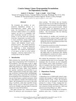
FORMULATING LINEAR PROGRAMMING MODELS

Session #4 Page 1
Formulating Linear Programming Models

Formulating Linear Programming Models

Some Examples:
• Product Mix (Session #2)
• Cash Flow (Session #3)
• Diet / Blending
• Scheduling
• Transportation / Distribution
• Assignment

Steps for Developing an Algebraic LP Model
1. What decisions need to be made? Define each decision variable.
2. What is the goal of the problem? Write down the objective function as a
function of the decision variables.
3. What resources are in short supply and/or what requirements must be met?
Formulate the constraints as functions of the decision variables.

Steps for Developing an LP Model in a Spreadsheet
1. Enter all of the data for the model. Make consistent use of rows and
columns.
2. Make a cell for each decision to be made (changing cells). Follow the same
structure as the data. (Sometimes it is easier to do step 2 before step 1.)
3. What is the goal of the problem? Enter the equation that measures the
objective in a single cell on the worksheet (target cell). Typically:

SUMPRODUCT (Cost Data, Changing Cells)
or

SUMPRODUCT (Profit Data, Changing Cells)

4. What resources are in short supply and/or what requirements must be met?
Enter all constraints in three consecutive cells on the spreadsheet, e.g.,

amount of resource used , <= , amount of resource available

Session #4 Page 2
Formulating Linear Programming Models

or
amount attained , >= , minimum requirement

Session #4 Page 3
Formulating Linear Programming Models

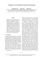
LP Example #1 (Diet Problem)

A prison is trying to decide what to feed its prisoners. They would like to offer
some combination of milk, beans, and oranges. Their goal is to minimize cost,
subject to meeting the minimum nutritional requirements imposed by law. The cost
and nutritional content of each food, along with the minimum nutritional
requirements are shown below.

Niacin (mg) Milk Navy Oranges Minimum
Thiamin (mg) (gallons) Beans (large Calif. Daily
Vitamin C (mg) (cups) Valencia)
3.2 Requirement
Cost ($) 1.12 4.9 0.8
32.0 1.3 0.19 13.0

0.0 93.0 1.5
2.00 45.0
0.20 0.25

Session #4 Page 4
Formulating Linear Programming Models

A Spreadsheet Model for LP Example #1

A B C D E F G H

1 The Prison Diet Problem

2

3 Milk Beans

4 (gal.) (cups) Oranges

5 Cost $2.00 $0.20 $0.25

6

7 Minimum

8 Nutritional Contents (mg) Total Requirement

9 Niacin (mg) 3.2 4.9 0.8 13 >= 13

10 Thiamin (mg) 1.12 1.3 0.19 3.438 >= 1.5

11 Vitamin C (mg) 32 0 93 45 >= 45

12

13 Total Cost
$0.64
14 Quantity 0 2.574 0.484

15 (per prisoner)

B C D E F G H

3 Milk Beans

4 (gal.) (cups) Oranges

5 Cost 2 0.2 0.25

6

7 Minimum
Requirement
8 Nutritional Contents (mg) Total

9 Niacin (mg) 3.2 4.9 0.8 =SUMPRODUCT(C9:E9,$C$14:$E$14) >= 13
>= 1.5
10 Thiamin (mg) 1.12 1.3 0.19 =SUMPRODUCT(C10:E10,$C$14:$E$14) >= 45

11 Vitamin C (mg) 32 0 93 =SUMPRODUCT(C11:E11,$C$14:$E$14)

12

13 Total Cost
=SUMPRODUCT(C5:E5,C14:E14)
14 Quantity 0 2.5740618802.84187368470967741935

15 (per prisoner)

Session #4 Page 5
Formulating Linear Programming Models

Diet/Menu Planning Model in Practice

George Dantzig’s Diet

• Stigler (1945) “The Cost of Subsistence”
• Dantzig invents the simplex method (1947)
• Stigler’s problem “solved” in 120 man days (1947)
• Dantzig goes on a diet (early 1950’s), applies diet model:

o ≤ 1500 calories
o objective: maximize (weight minus water content)
o 500 foods
• Initial solutions had problems (500 gallons of vinegar, 200 bouillon cubes)

(for more details, see July-Aug 1990 Interfaces article “The Diet Problem”, available for download at
under “Published Issues”)

Least-Cost Menu Planning Models in Food Systems Management

• Used in many institutions with feeding programs: hospitals, nursing homes,
schools, prisons, etc.

• Menu planning often extends to a sequence of meals or cycle
• Variety important (separation constraints)
• Preference ratings (related to service frequency)
• Side constraints (color, categories, etc.)
• Generally models have reduced cost about 10%, meet nutritional

requirements better, and increased customer satisfaction compared to
traditional methods
• USDA uses these models to plan food stamp allotment

(for more details, see Sept-Oct 1992 Interfaces article “The Evolution of the Diet Model in Managing Food
Systems”, available for download at under “Published Issues”)

Session #4 Page 6
Formulating Linear Programming Models

LP Example #2 (Scheduling Problem)

Time Period Number of
Officers
12 a.m. - 4 a.m. Needed
4 a.m. - 8 a.m.
8 a.m. - 12 p.m. 5
12 p.m. - 4 p.m. 7
4 p.m. - 8 p.m. 15
8

8 p.m. - 12 a.m. 12

9

Union contract requires all employees to work 8 consecutive hours.
Goal: Hire the minimum number of officers needed to cover all shifts.

Session #4 Page 7
Formulating Linear Programming Models

A Spreadsheet Model for LP Example #2

A B C D E F G H I J K

1 Security Force Scheduling Problem

2

3 Shift Works Time Period?

4 Shift 1 Shift 2 Shift 3 Shift 4 Shift 5 Shift 6 Number Minimum

5 Time Period 12a–8a 4a–12p 8a–4p 12p–8p 4p–12a 8p–4a Working Required

6 12am – 4am 1 1 5 >= 5

7 4am – 8am 1 1 12 >= 7

8 8am – 12pm 1 1 15 >= 15

9 12pm – 4pm 1 1 8 >= 8

10 4pm – 8pm 1 1 12 >= 12

11 8pm – 12am 1 1 12 >= 9

12

13 Total

14 Number Working 5 7 8 0 12 0 32

B C D E F G H I J K

3 Shift Works Time Period?

4 Shift 1 Shift 2 Shift 3 Shift 4 Shift 5 Shift 6 Number Minimum

5 Time Period 12a–8a 4a–12p 8a–4p 12p–8p 4p–12a 8p–4a Working Required

6 12am – 4am 1 1 =SUMPRODUCT(C6:H6,$C$14:$H$14) >= 5

7 4am – 8am 1 1 =SUMPRODUCT(C7:H7,$C$14:$H$14) >= 7

8 8am – 12pm 1 1 =SUMPRODUCT(C8:H8,$C$14:$H$14) >= 15

9 12pm – 4pm 1 1 =SUMPRODUCT(C9:H9,$C$14:$H$14) >= 8

10 4pm – 8pm 1 1 =SUMPRODUCT(C10:H10,$C$14:$H$14) >= 12

11 8pm – 12am 1 1 =SUMPRODUCT(C11:H11,$C$14:$H$14) >= 9

12

13 Total

14 Number Working 5 7 8 0 12 0 =SUM(C14:H14)

Session #4 Page 8
Formulating Linear Programming Models

Workforce Scheduling Model in Practice

United Airlines in the 1980’s
• Employ 5000 reservation and customer service agents
• Some part time (2-8 hr shifts), some full time (8-10 hour shifts)
• Workload varies greatly over day
• Modeled problem as LP:
o Decision variables: how many employees of each shift length should
begin at each potential start time (half-hour intervals).
o Constraints: minimum required employees for each half-hour
o Objective: minimize cost
• Saved UA about $6 million annually, improved customer service, still in use
today.

(for more details, see Jan-Feb 1986 Interfaces article “United Airlines Station Manpower Planning System”,
available for download at under “Published Issues”)

Session #4 Page 9
Formulating Linear Programming Models

LP Example #3 (Transportation Problem)

A company has two plants producing a certain product that is to be shipped to three
distribution centers. The unit production costs are the same at the two plants, and
the shipping cost per unit is shown below.

Plant Distribution
Center

1 2 3
A $4 $6 $4

B $6 $5 $2

Shipments are made once per week. During each week, each plant produces at
most 60 units and each distribution center needs at least 40 units. How many units
should be shipped from each plant to each distribution center, so as to minimize
cost?

Session #4 Page 10
Formulating Linear Programming Models

Spreadsheet Model for LP Example #3

A B C D E F G H

1 A Distribution Problem

2

3 Distribution Distribution Distribution
Center 3
4 Cost Center 1 Center 2 $4
$2
5 Plant A $4 $6

6 Plant B $6 $5

7

8

9

10

11 Shipment Distribution Distribution Distribution
Center 3
12 Quantities Center 1 Center 2 0 Shipped Available
40 60
13 Plant A 40 20 40 60 <= 60
>=
14 Plant B 0 20 60 <=
40
15 Shipped 40 40

16 >= >= Total Cost
$460
17 Needed 40 40

B C D E F G H

3 Distribution Distribution Distribution

4 Cost Center 1 Center 2 Center 3

5 Plant A 4 6 4

6 Plant B 6 5 2

7

8

9

10

11 Shipment Distribution Distribution Distribution

12 Quantities Center 1 Center 2 Center 3 Shipped Available

13 Plant A 40 20 0 =SUM(C13:E13) <= 60

14 Plant B 0 20 40 =SUM(C14:E14) <= 60

15 Shipped =SUM(C13:C14) =SUM(D13:D14) =SUM(E13:E14)

16 >= >= >= Total Cost

17 Needed 40 40 40 =SUMPRODUCT(C5:E6,C13:E14)

Session #4 Page 11
Formulating Linear Programming Models

Designing a Distribution System for Entire Product Line
(Proctor and Gamble)

Proctor and Gamble in early 90’s
• Needed to consolidate and re-design their North American distribution system:
o 50 product categories
o 60 plants
o 15 distribution centers
o 1000 customer zones

• Solved many transportation problems (1 for each product category)

• Goal: find best distribution plan, which plants to keep open, etc.

• Saved $200 million per year.

(for more details, see 1997 Jan-Feb Interfaces article, “Blending OR/MS, Judgement, and GIS: Restructuring P&G’s
Supply Chain”, available for download at under “Published Issues”)

Session #4 Page 12
Formulating Linear Programming Models

LP Example #4 (Assignment Problem)

The coach of a swim team needs to assign swimmers to a 200-yard medley relay
team (four swimmers, each swims 50 yards of one of the four strokes). Since most
of the best swimmers are very fast in more than one stroke, it is not clear which
swimmer should be assigned to each of the four strokes. The five fastest swimmers
and their best times (in seconds) they have achieved in each of the strokes (for 50
yards) are

Carl Backstroke Breaststroke Butterfly Freestyle

Chris 37.7 43.4 33.3 29.2
David
Tony 32.9 33.1 28.5 26.4
Ken 33.8 42.2 38.9 29.6
37.0 34.7 30.4 28.5
34.4 41.8 32.8 31.1

How should the swimmers be assigned to make the fastest relay team?

Session #4 Page 13
Formulating Linear Programming Models

Spreadsheet Model for LP Example #4

A B C D E F GH I

1 An Assignment Problem Butterfly
33.3
2 28.5
38.9
3 Best Times Backstroke Breastroke 30.4 Freestyle

33.6 29.2
4 Carl 37.7 43.4 26.4
Butterfly 29.6
5 Chris 32.9 33.1 0 28.5
1 31.1
6 David 33.8 42.2 0
0
7 Tony 37.0 34.7 0
1
8 Ken 34.4 41.8 =
1
9

10

11 Assignment Backstroke Breastroke Freestyle
1
12 Carl 0 0 0 1 <= 1
0 1 <= 1
13 Chris 0 0 0 1 <= 1
0 1 <= 1
14 David 1 0 1 0 <= 1
=
15 Tony 0 1 Time
1 126.2
16 Ken 0 0

17 1 1

18 = =

19 1 1

B C D E F G H I

3 Best Times Backstroke Breastroke Butterfly Freestyle
43.4 33.3 29.2
4 Carl 37.7 33.1 28.5 26.4
42.2 38.9 29.6
5 Chris 32.9 34.7 30.4 28.5
41.8 33.6 31.1
6 David 33.8

7 Tony 37

8 Ken 34.4

9

10

11 Assignment Backstroke Breastroke Butterfly Freestyle

12 Carl 0 0 0 1 =SUM(C12:F12) <= 1

13 Chris 0 0 1 0 =SUM(C13:F13) <= 1

14 David 1 0 0 0 =SUM(C14:F14) <= 1

15 Tony 0 1 0 0 =SUM(C15:F15) <= 1

16 Ken 0 0 0 0 =SUM(C16:F16) <= 1

17 =SUM(C12:C16) =SUM(D12:D16) =SUM(E12:E16) =SUM(F12:F16)

18 = = = = Time

19 1 1 1 1 =SUMPRODUCT(C4:F8,C12:F16)