Advances in Greedy Algorithms_1 docx
Bạn đang xem bản rút gọn của tài liệu. Xem và tải ngay bản đầy đủ của tài liệu tại đây (28.02 MB, 300 trang )
Advances in Greedy Algorithms
Advances in Greedy Algorithms
Edited by
Witold Bednorz
I-Tech
IV
Published by In-Teh
In-Teh is Croatian branch of I-Tech Education and Publishing KG, Vienna, Austria.
Abstracting and non-profit use of the material is permitted with credit to the source. Statements and
opinions expressed in the chapters are these of the individual contributors and not necessarily those of
the editors or publisher. No responsibility is accepted for the accuracy of information contained in the
published articles. Publisher assumes no responsibility liability for any damage or injury to persons or
property arising out of the use of any materials, instructions, methods or ideas contained inside. After
this work has been published by the In-Teh, authors have the right to republish it, in whole or part, in
any publication of which they are an author or editor, and the make other personal use of the work.
© 2008 In-teh
www.in-teh.org
Additional copies can be obtained from:
First published November 2008
Printed in Croatia
A catalogue record for this book is available from the University Library Rijeka under no. 120115050
Advances in Greedy Algorithms, Edited by Witold Bednorz
p. cm.
ISBN 978-953-7619-27-5
1. Advances in Greedy Algorithms, Witold Bednorz
Preface
The greedy algorithm is one of the simplest approaches to solve the optizmization
problem in which we want to determine the global optimum of a given function by a
sequence of steps where at each stage we can make a choice among a class of possible
decisions. In the greedy method the choice of the optimal decision is made on the
information at hand without worrying about the effect these decisions may have in the
future. Greedy algorithms are easy to invent, easy to implement and most of the time quite
efficient. However there are many problems that cannot be solved correctly by the greedy
approach. The common example of the greedy concept is the problem of ‘Making Change’
in which we want to make a change of a given amount using the minimum number of US
coins. We can use five different values: dollars (100 cents), quarters (25 cents), dimes (10
cents), nickels (5 cents) and pennies (1 cent). The greedy algorithm is to take the largest
possible amount of coins of a given value starting from the highest one (100 cents). It is easy
to see that the greedy strategy is optimal in this setting, indeed for proving this it suffices to
use the induction principle which works well because in each step either the procedure has
ended or there is at least one coin we can use of the actual value. It means that the problem
has a certain optimal substructure, which makes the greedy algorithm effective. However a
slight modification of ‘Making Change’, e.g. where one value is missing, may turn the
greedy strategy to be the worst choice. Therefore there are obvious limits for using the
greedy method: whenever there is no optimal substructure of the problem we cannot hope
that the greedy algorithm will work. On the other hand there is a lot of problems where the
greedy strategy works unexpectedly well and the purpose of this book is to communicate
various results in this area. The key point is the simplicity of the approach which makes the
greedy algorithm a natural first choice to analyze the given problem. In this book there are
discussed several algorithmic questions in: biology, combinatorics, networking, scheduling
or even pure mathematics, where the greedy algorithm can be used to produce the optimal
or nearly optimal answer.
The book was written in 2008 by the numerous authors who contributed the publication
by presenting their researches in a form of a self-contained chapters. The idea was to
coordinate the international project where specialists all over the world can share their
knowledge on the greedy algorithms theory. Each chapter comprises a separate study on
some optimization problem giving both an introductory look into the theory the problem
comes from and some new developments invented by author(s). Usually some elementary
knowledge is assumed, yet all the required facts are quoted mostly in examples, remarks or
theorems. The publication may be useful for all graduates and undergraduates interested in
the algorithmic theory with the focus on the greedy approach and applications of this
VI
method to various concrete examples. Most of scientists involved in the project are young at
the full strength of their career, hence the presented content is fresh and acquaints with the
new directions where the theory of greedy algorithms evolves to.
On the behalf of authors I would like to acknowledge all who made the publication
possible, in particular to Vedran Kordic who coordinated this huge project. Many thanks
also for those who helped in the manuscripts preparation making useful suggestions and
finding errors.
November 2008
Editor
Witold Bednorz
Warsaw,
Poland,
Contents
Preface V
1. A Greedy Algorithm with Forward-Looking Strategy 001
Mao Chen
2. A Greedy Scheme for Designing Delay Monitoring Systems
of IP Networks
017
Yigal Bejerano and Rajeev Rastogi
3. A Multilevel Greedy Algorithm for the Satisfiability Problem 039
Noureddine Bouhmala and Xing Cai
4. A Multi-start Local Search Approach to the Multiple Container
Loading Problem
055
Shigeyuki Takahara
5. A Partition-Based Suffix Tree Construction and Its Applications 69
Hongwei Huo and Vojislav Stojkovic
6. Bayesian Framework for State Estimation and Robot Behaviour
Selection in Dynamic Environments
85
Georgios Lidoris, Dirk Wollherr and Martin Buss
7. Efficient Multi-User Parallel Greedy Bit-Loading Algorithm with
Fairness Control For DMT Systems
103
Cajetan M. Akujuobi and Jie Shen
8. Energy Efficient Greedy Approach for Sensor Networks 131
Razia Haider and Dr. Muhammad Younus Javed
9. Enhancing Greedy Policy Techniques for Complex
Cost-Sensitive Problems
151
Camelia Vidrighin Bratu and Rodica Potolea
VIII
10. Greedy Algorithm: Exploring Potential of Link Adaptation Technique
in Wideband Wireless Communication Systems
169
Mingyu Zhou, Lihua Li, Yi Wang and Ping Zhang
11. Greedy Algorithms for Mapping onto a Coarse-grained
Reconfigurable Fabric
193
Colin J. Ihrig, Mustafa Baz, Justin Stander, Raymond R. Hoare, Bryan A. Norman,
Oleg Prokopyev, Brady Hunsaker and Alex K. Jones
12. Greedy Algorithms for Spectrum Management in OFDM Cognitive
Systems - Applications to Video Streaming and Wireless Sensor Networks
223
Joumana Farah and François Marx
13. Greedy Algorithms in Survivable Optical Networks 245
Xiaofei Cheng
14. Greedy Algorithms to Determine Stable Paths and Trees
in Mobile Ad hoc Networks
253
Natarajan Meghanathan
15. Greedy Anti-Void Forwarding Strategies for Wireless Sensor Networks 273
Wen-Jiunn Liu and Kai-Ten Feng
16. Greedy Like Algorithms for the Traveling Salesman
and Multidimensional Assignment Problems
291
Gregory Gutin and Daniel Karapetyan
17. Greedy Methods in Plume Detection, Localization and Tracking 305
Huimin Chen
18. Greedy Type Bases in Banach Spaces 325
Witold Bednorz
19. Hardware-oriented Ant Colony Optimization Considering
Intensification and Diversification
359
Masaya Yoshikawa
20. Heuristic Algorithms for Solving Bounded Diameter Minimum Spanning
Tree Problem and Its Application to Genetic Algorithm Development
369
Nguyen Duc Nghia and Huynh Thi Thanh Binh
21. Opportunistic Scheduling for Next Generation Wireless
Local Area Networks
387
Ertuğrul Necdet Çiftçioğlu and Özgür Gürbüz
IX
22. Parallel Greedy Approximation on Large-Scale Combinatorial Auctions 411
Naoki Fukuta and Takayuki Ito
23. Parallel Search Strategies for TSPs using a Greedy Genetic Algorithm 431
Yingzi Wei and Kanfeng Gu
24. Provably-Efficient Online Adaptive Scheduling of Parallel Jobs
Based on Simple Greedy Rules
439
Yuxiong He
and Wen-Jing Hsu
25. Quasi-Concave Functions and Greedy Algorithms 461
Yulia Kempner, Vadim E. Levit and Ilya Muchnik
26. Semantic Matchmaking Algorithms 481
Umesh Bellur and Harin Vadodaria
27. Solving Inter-AS Bandwidth Guaranteed Provisioning Problems
with Greedy Heuristics
503
Kin-Hon Ho, Ning Wang and George Pavlou
28. Solving the High School Scheduling Problem Modelled
with Constraints Satisfaction using Hybrid Heuristic Algorithms
529
Ivan Chorbev, Suzana Loskovska, Ivica Dimitrovski and Dragan Mihajlov
29. Toward Improving b-Coloring based Clustering
using a Greedy re-Coloring Algorithm
553
Tetsuya Yoshida, Haytham Elghazel, Véronique Deslandres,
Mohand-Said Hacid and Alain Dussauchoy
30. WDM Optical Networks Planning using Greedy Algorithms 569
Nina Skorin-Kapov
1
A Greedy Algorithm with
Forward-Looking Strategy
Mao Chen
Engineering Research Center for Educational Information Technology,
Huazhong Normal University,
China
1. Introduction
The greedy method is a well-known technique for solving various problems so as to
optimize (minimize or maximize) specific objective functions. As pointed by Dechter et al
[1], greedy method is a controlled search strategy that selects the next state to achieve the
largest possible improvement in the value of some measure which may or may not be the
objective function. In recent years, many modern algorithms or heuristics have been
introduced in the literature, and many types of improved greedy algorithms have been
proposed. In fact, the core of many Meta-heuristic such as simulated annealing and genetic
algorithms are based on greedy strategy.
“The one with maximum benefit from multiple choices is selected” is the basic idea of
greedy method. A greedy method arrives at a solution by making a sequence of choices,
each of which simply looks the best at the moment. We refer to the resulting algorithm by
this principle the basic greedy (BG) algorithm, the details of which can be described as
follow:
Procedure BG (partial solution S, sub-problem P)
Begin
generate all candidate choices as list L for current sub-problem P;
while (L is not empty OR other finish condition is not met)
compute the fitness value of each choice in L;
modify S and P by taking the choice with highest fitness value;
update L according to S and P;
end while;
return the quality of the resulting complete solution;
End.
For an optimization problem, what remains is called a sub-problem after making one or
several steps of greedy choice. For problem or sub-problem P, let S be the partial solution,
and L be the list of candidate choices at the current moment.
To order or prioritize the choices, some evaluation criteria are used to express the fitness
value. According to the BG algorithm, the candidate choice with the highest fitness value is
selected, and the partial solution is updated accordingly. This procedure repeated step by
step until a resulting complete solution is obtained.
Advances in Greedy Algorithms
2
The representation of the BG algorithm can be illustrated by a search tree as shown in Fig.1.
Each node in the search tree corresponds to a partial solution, and a line between two nodes
represents the decision to add a candidate choice to the existing partial solution.
Consequently, leaf nodes at the end of tree correspond to complete solutions.
In Fig.1, the black circle at level 1 denotes an initial partial solution. At level 2, there are four
candidate choices for current partial solution, which denotes by four nodes. In order to
select the best node, promise of each node should be determined. After some evaluation
function has been employed, the second node with highest benefit (the circle in gray at level
2) is selected. Then, the partial solution and sub-problem are updated accordingly.
Fig. 1. Representation of basic greedy algorithm
Two important features of greedy method make it so popular are simple implementation and
efficiency. Simple as it is, BG algorithm is highly efficient and sometimes it can produce an
optimal solution for some optimization problem. For example, for problems such as activity-
selection problem, fractional knapsack problem and minimum spanning trees problem, BG
algorithm can obtain optimal solution by making a series of greedy choice. For these problems
that the BG algorithm can obtain optimal solution, there is something in common: the optimal
solution to the problem contains within it optimal solutions to sub-problems.
However, for other optimization problems that do not exhibit such property, the BG
algorithm will not lead to optimal solution. Especially for the combinatorial optimization
problems or NP-hard problem, the solution by BG algorithm is far away from satisfactory.
A Greedy Algorithm with Forward-Looking Strategy
3
In BG algorithm, we make whatever choice seems best at the moment and then turn to solve
the sub-problem arising after the choice is made. That is to say, the benefit is only locally
evaluated. Consequently, even though we select the best at each step, we still missed the
optimal solution. Just liking playing chess, a player who is focused entirely on immediate
advantage is easy to be defeated, the player who can think several step ahead will win with
more opportunity.
In this chapter, a novel greedy algorithm is introduced in detail, which is of some degree of
forward-looking. In this algorithm, all the choices at the moment are evaluated more
globally before the best one is selected. The greedy idea and enumeration strategy are both
reflected in this algorithm, and we can adjust the enumeration degree so we can balance the
efficiency and speed of algorithm.
2. Greedy Algorithm with forward-looking search strategy
To evaluate the benefit of a candidate choice more globally, an improved greedy algorithm
with forward-looking search strategy (FG algorithm) was proposed by Huang et al [2],
which was first proposed for tackling packing problem. It is a kind of growth algorithm and
it is efficient for problem that can be divided into a series of sub-problems.
In FG algorithm, the promise of a candidate choice is evaluated not only by the current
circumstance, but more globally by considering the quality of the complete solution that can
be obtained from the partial solution represented by the node. The idea of FG algorithm can
be illustrated by Fig.2:
Fig. 2. Representation of greedy algorithm with forward-looking strategy
Advances in Greedy Algorithms
4
As shown in Fig.2 (a), there are four nodes at level 2 for the initial partial solution. We do
not evaluate the promise of each node at once at the moment. Conversely, we tentatively
update the initial partial solution by take the choices at level 2 respectively. For each node at
level 2 (i.e., each partial solution at level 2), its benefit is evaluated by the quality of the
complete solution resulted from it according to BG algorithm. From the complete solution
with maximum quality, we backtrack it to the partial solution and definitely take this step.
In other words, the node that corresponds to the complete solution with maximum quality
(the gray circle in Fig.2 (a)) is selected as the partial solution. Then the search progresses to
level 3. Level by level, this process is repeated until a complete solution is obtained.
After testing the global benefit of each node at current level, the one with great prospect will
be selected. This idea can be referred as forward-looking, or backtracking. More formally,
the procedure above can be described as follows:
Procedure FG (problem P)
Begin
generate the initial partial solution S, and update P to a sub-problem;
generate all current candidate choice as a list L;
while (L is not empty AND finish condition is not met)
max
⇐0
for each choice c in L
compute the global benefit: GloableBenefit (c, S, P);
update max with the benefit;
end for;
modify S by selecting the choice that the global benefit equal to max;
update P and L;
end while;
End.
As shown in the above algorithm, in order to more globally evaluate the benefit of a choice
and to overcome the limit of BG algorithm, we compute the benefit of a choice using BG
itself in the procedure GlobalBenefit
to obtain the so-called FG algorithm
.
Similarly to BG algorithm, we start from the initial partial solution and repeat the above
procedure until a complete solution is reached. Note that if there are several complete
solutions with the same maximum benefit, we will select the first one to break the tie.
The global benefit of each candidate choice is described as:
Procedure GlobalBenefit (choice c, partial solution S, sub-problem P)
Begin
let S’and P’ be copies of S and P;
modify S’and P’ by taking the choice c;
return BG(S, P);
End.
Given a copy S’ of the partial solution and a copy P’of sub-problem, then we update S’by
taking the choice c. For the resulted partial solution and sub-problem, we use BG algorithm
to obtain the quality of the complete solution.
It should be noted that Procedure FG only gives one initial partial solution. For some
problems, there may be several choices for the initial partial solution. Similarly, the
A Greedy Algorithm with Forward-Looking Strategy
5
Procedure globalBenefit() is implemented for the initial partial solutions respectively, and the
one with maximum benefit should be selected.
3. Improved version of FG algorithm
3.1 Filtering mechanism
For some problems, the number of nodes is rather large at each level of search. Therefore, a
filtering mechanism is proposed to reduce the computational burden. During filtering some
nodes will not be given chance to be evaluated globally and be discarded permanently based
on their local evaluation value. Only the remaining nodes are subject to global evaluation.
Fig. 3. Representation of filtering mechanism
As shown in Fig.3, there are 7 nodes at level 2. Firstly, the benefit of each node is locally
evaluated. Then, only the promising nodes whose local benefit is larger than a given
threshold parameter
τ
will be globally evaluated. The FG algorithm can be modified as
FGFM algorithm:
Advances in Greedy Algorithms
6
Procedure FGFM (problem P)
Begin
generate the initial partial solution S, update P to a sub-problem;
generate all current candidate choice as a list L;
while (L is not empty AND finish condition is not met)
max
⇐0
for each choice c in L
if (local benefit > parameter
τ
)
compute the global benefit: GloableBenefit (c, S, P);
update max with global benefit;
end if;
end for;
modify S by selecting the choice that the global benefit equal to max;
update P and L;
end while;
End.
Obviously, the threshold parameter
τ
is used to control the trade-off between the quality of
the result and the computational time. If
τ
is set to be large enough, algorithm FGFM turns
to be a BG algorithm; If
τ
is set to be small enough, algorithm FGFM turns to be a FG
algorithm.
3.2 Multiple level enumerations
In the FG algorithm, the benefit of a node is globally evaluated by the quality of
corresponding complete solution, which is resulted from the node level by level according
to the BG algorithm. In order to further improve the quality of the solution, the forward-
looking strategy can be applied to several levels.
This multi-level enumeration can be illustrated by Fig.4. For the initial partial solution, there
are three candidate choices at level 2. From each node at level 2, there are several branches
at level 3. Then we use procedure GlobalBenefit () to evaluate the global benefit of each nodes
at level 3. That is to say, the three nodes at level 2 have several global benefits. We will
choose the highest one as its global benefit. Afterwards, the one with the maximum global
benefit from the three nodes at level 2 are selected as the partial solution.
If the number of enumeration levels is equal to (last level number - current level number-1)
for each node, the search tree will become a complete enumeration tree, the corresponding
solution of which will surely be optimal solution. However, the computational time
complexity is unacceptable. Usually, the number of enumeration levels ranges from 1 to 4.
Obviously, the filtering mechanism and multi-level enumeration strategy are the means to
control the trade-off between solution quality and runtime effort.
4. Applications
FG algorithm has been successfully applied to job shop scheduling problem [3], circle
packing problem [2, 4] and rectangular packing problem [5]. In this section, the two-
dimensional (2D) rectangle packing problem and its corresponding bounded enumeration
algorithm is presented.
A Greedy Algorithm with Forward-Looking Strategy
7
backtracking
Fig. 4. The multi-level enumeration strategy
4.1 Problem definition
The 2D rectangular packing problem has been widely studied in recent decades, as it has
numerous applications in the cutting and packing industry, e.g. wood, glass and cloth
industries, newspapers paging, VLSI floor planning and so on, with different applications
incorporating different constraints and objectives.
We consider the following rectangular packing problem: given a rectangular empty
container with fixed width and infinite height and a set of rectangles with various sizes, the
rectangle packing problem is to pack each rectangle into the container such that no two
rectangles overlap and the used height of the container is minimized. From this
optimization problem, an associated decision problem can be formally stated as follows:
Given a rectangular board with given width W and given height H, and n rectangles with
length li and width wi, 1
≤
i
≤
n, take the origin of the two-dimensional Cartesian coordinate
system at the bottom-left corner of the container (see Fig.5). The aim of this problem is to
determine if there exist a solution composed of n sets of quadruples
11 11 12 12
{, , , }
x
yxy ,…,
112 2
{, , , }
nnn n
x
yx y , where (
11
,
ii
x
y ) denotes the bottom-left corner coordinates of rectangle i,
and (
22
,
ii
x
y ) denotes the top-right corner coordinates of rectangle i. For all 1 ≤ i ≤ n, the
coordinates of rectangle i satisfy the following conditions:
1. x
i2
−x
i1
= l
i
∧ y
i2
−y
i1
= w
i
or x
i2
−x
i1
= w
i
∧ y
i2
−y
i1
= l
i
;
Advances in Greedy Algorithms
8
2. For all 1
≤ i, j
≤
n, j
≠
i, rectangle i and j cannot overlap, i.e., one of the following
condition should be met: x
i1
≥
x
j2
or x
j
1
≥
x
i
2 or y
i1
≥
y
j2
or y
j
1
≥
y
i
2;
3. 0
≤ x
i1
, x
i
2 ≤ W and 0
≤
y
i1
, y
i2
≤
H.
In our packing process, each rectangle is free to rotate and its orientation
θ
can be 0 (for “not
rotated”) or 1 (for “rotated by
π
/2”). It is noted that the orthogonal rectangular packing
problems denote that the packing process has to ensure the edges of each rectangle are
parallel to the x- and y-axis, respectively.
Obviously, if we can find an efficient algorithm to solve this decision problem, we can then
solve the original optimization problem by using some search strategies. For example, we
first apply dichotomous search to get rapidly a “good enough” upper bound for the height,
then from this upper bound we gradually reduce it until the algorithm no longer finds a
successful solution. The final upper bound is then taken as the minimal height of the
container obtained by the algorithm. In the following discussion, we will only concentrate
on the decision problem of fixed container.
O
(x
i2
,y
i2
)
y
(x
i1
,y
i1
)
x
R
i
Fig. 5. Cartesian coordinate system
4.2 Preliminary
Definition Configuration. A configuration C is a pattern (layout) where m (0 mn≤<)
rectangles have been already packed inside the container without overlap, and n
−m
rectangles remain to be packed into the container.
A configuration is said to be successful if m=n, i.e., all the rectangles have been placed inside
the container without overlapping. A configuration is said to be failure if m<n and none of
the rectangles outside the container can be packed into the container without overlapping. A
configuration is said final if it is either a successful configuration or a failure configuration.
Definition Candidate corner-occupying action. Given a configuration with m rectangles
packed, there may be many empty corners formed by the previously packed rectangles and
the four sides of the container. Let rectangle i be the current rectangle to be packed, a
candidate corner-occupying action (CCOA) is the placement of rectangle i at an empty
corner in the container so that rectangle i touches the two items forming the corner and does
A Greedy Algorithm with Forward-Looking Strategy
9
not overlap other previously packed rectangles (an item may be a rectangle or one of the
four sides of the container). Note that the two items are not necessarily touching each other.
Obviously, the rectangle to be packed has two possible orientation choices at each empty
corner, that is, the rectangle can be placed with its longer side laid horizontally or vertically.
A CCOA can be represented by a quadri-tuple (i, x, y,
θ
), where (x, y) is the coordinate of the
bottom-left corner of the suggested location of rectangle i and
θ
is the corresponding
orientation.
R
1
R
4
R
3
R
2
2
3
5
1
4
Fig. 6. Candidate corner-occupying action for rectangle R
4
Under current configuration, there may be several candidate packing positions for the
current rectangle to be packed. At the configuration in Fig.6, three rectangles R
1
, R
2
and R
3
are already placed in the container. There are totally 5 empty corners to pack rectangle R
4
,
and R
4
can be packed at any one of them with two possible orientations. As a result, there
are 10 CCOAs for R
4.
In order to prioritize the candidate packing choices, we need a concept that expresses the
fitness value of a CCOA. Here, we introduce the quantified measure
λ
, called degree to
evaluate the fitness value of a CCOA. Before presenting the definition of degree, we first
introduce the definition of minimal distance between rectangles as follows.
R
1
R
2
R
3
Fig. 7. Illustration of distance
Definition Minimal distance between rectangles. Let i
and j be two rectangles already placed in
the container, and (x
i
, y
i
), (x
j
, y
j
) are the coordinates of arbitrary point on rectangle i
and j,
respectively. The minimal distance d
ij
between i
and j is:
Advances in Greedy Algorithms
10
22
min{ ( ) ( ) }
ij i j i j
dxxyy=−+−
In Fig.7, R
3
is packed on the position occupying the corner formed by the upper side and the
right side of the container. As shown in Fig.7, the minimal distance between R
3
and R
1
, and
the minimal distance between R
3
and R
2
are illustrated, respectively.
Definition Degree of CCOA. Let M be the set of rectangles already placed in the container.
Rectangle i is the current rectangle to be packed, (i, x, y,
θ
) is one of the CCOAs for rectangle
i. If corner-occupying action (i, x, y,
θ
) places rectangle i at a corner formed by two items
(rectangle or side of the container) u and v, the degree
λ
of the corner-occupying action (i, x,
y,
θ
) is defined as:
min
1()
2
ii
wl
d
λ
+
=− /
where w
i
and l
i
are the width and the length of rectangle i, and d
min
is the minimal distance
from rectangle i to other rectangles in M and sides of the container (excluding u and v), that
is,
min 1234
min{ | { , , , }, , }
ij
ddjMssssjuv=∈ ≠∪
where s
1
, s
2
, s
3
and s
4
are the four sides of the container.
It is clear that if a corner-occupying action place rectangle i at a position very close to the
previously packed rectangles, the corresponding degree will be very high. Note that, if
rectangle i can be packed by a CCOA at a corner in the container and touches more than two
items, then d
min
=0 and
λ
=1; otherwise
λ
<1. The degree of a corner-occupying action
describes how the placed rectangle is close to the already existing pattern. Thus, we use it as
the benefit of a packing step.
Intuitively, since one should place a rectangle as close as possible to the already existing
pattern, it seems quite natural that the CCOA with the highest degree will be selected first to
pack the rectangle into the container. We call this principle the highest degree first (HDF)
rule. It is just the simple application of BG algorithm.
4.3 The basic algorithm: A
0
Based on the HDF rule and BG algorithm, A
0
is described as follows:
Procedure A
0
(C, L)
Begin
while (L is not empty)
for each CCOA in L
calculate the degree;
end for;
select the CCOA (i, x, y,
θ
) with the highest degree;
modify C by placing rectangle i at (x, y) with orientation
θ
;
modify L according to the new configuration C;
end while;
return C;
End.
A Greedy Algorithm with Forward-Looking Strategy
11
At each iteration, a set of CCOAs for each of the unpacked rectangles is generated under
current configuration C. Then the CCOAs for all the unpacked rectangles outside the
container are gathered as a list L. A
0
calculates the degree of each CCOA in L and selects the
CCOA (i, x, y,
θ
) with the highest degree
λ
, and place rectangle i at (x, y) with orientation
θ
.
After placing rectangle i, the list L is modified as follows:
1. Remove all the CCOAs involving rectangle i;
2. Remove all infeasible CCOAs. A CCOA becomes infeasible because the involved
rectangle would overlap rectangle i if it was placed;
3. Re-calculate the degree
λ
of the remaining CCOAs;
4. If a rectangle outside the container can be placed inside the container without overlap
so that it touches rectangle i and a rectangle inside the container or the side of the
container, create a new CCOA and put it into L, and compute the degree
λ
of the new
CCOA.
If none of the rectangles outside the container can be packed into the container without
overlap (L is empty) at certain iteration, A
0
stops with failure (returns a failure
configuration). If all rectangles are packed in the container without overlap, A
0
stops with
success (returns a successful configuration).
It should be pointed out that if there are several CCOAs with the same highest degree, we
will select one that packs the corresponding rectangle closest to the bottom left corner of the
container.
A
0
is a fast algorithm. However, given a configuration, A
0
only considers the relation
between the rectangles already inside the container and the rectangle to be packed. It
doesn’t examine the relation between the rectangles outside the container. In order to more
globally evaluate the benefit of a CCOA and to overcome the limit of A
0
, we compute the
benefit of a CCOA using A
0
itself in the procedure BenefitA
1
to obtain our main packing
algorithm called A
1.
4.4 The greedy algorithm with forward-looking strategy: A
1
Based on current configuration C, CCOAs for all unpacked rectangles are gathered as a list
L. For each CCOA (i, x, y,
θ
) in L, the procedure BenefitA
1
is designed to evaluate its benefit
more globally.
Procedure BenefitA
1
(i, x, y,
θ
, C, L)
Begin
let C’and L’be copies of C and L;
modify C’by placing rectangle i at (x, y) with orientation
θ
, and modify L’;
C’= A
0
(C’,L’);
if (C’is a successful configuration)
Return C’;
else
Return density (C’);
end if-else
End.
Given a copy C’ of the current configuration C and a CCOA (i, x, y,
θ
) in L, BenefitA
1
begins
by packing rectangle i in the container at (x, y) with orientation
θ
and call A
0
to reach a final
configuration. If A
0
stops with success then BenefitA
1
returns a successful configuration,
Advances in Greedy Algorithms
12
otherwise BenefitA
1
returns the density (the ratio of the total area of the rectangles inside the
container to the area of the container) of a failure configuration as the benefit of the CCOA
(i, x, y,
θ
). In this manner, BenefitA
1
evaluates all existing CCOAs in L.
Now, using the procedure BenefitA
1
, the benefit of a CCOA is measured by the density of a
failure configuration. The main algorithm A
1
is presented as follow:
Procedure A
1
( )
Begin
generate the initial configuration C;
generate the initial CCOA list L;
while (L is not empty)
maximum benefit
←
0
for each CCOA (i, x, y,
θ
) in L
d= BenefitA
1
(i, x, y,
θ
, C, L);
if (d is a successful configuration)
stop with success;
else
update the maximum benefit with d;
end if-else;
end for;
select the CCOA (
*
i ,
*
x
,
*
y
,
*
θ
) with the maximum benefit;
modify C by placing rectangle
*
i at (
*
x
,
*
y
) with orientation
*
θ
;
modify L according to the new configuration C;
end while;
stop with failure
End.
Similarly, A
1
selects the CCOA with the maximum benefit and packs the corresponding
rectangle into the container by this CCOA at each iteration. If there are several CCOAs with
the maximum benefit, we select one that packs the corresponding rectangle closest to the
bottom left corner of the container.
4.5 Computational complexity
We analysis the complexity of A
1
in the worst case, that is, when it cannot find successful
configuration, and discuss the real computational cost to find a successful configuration.
A
0
is clearly polynomial. Since every pair of rectangles or sides in the container can give a
possible CCOA for a rectangle outside the container, the length of L is bounded by
O(m
2
(n−m)), if m rectangles are already placed in the container. For each CCOA in L, d
min
is
calculated using the d
min
in the last iteration in O(1) time. The creation of new CCOAs and
the calculus of their degree is also bounded by O(m
2
(n−m)) since there are at most
O(m(n−m)) new CCOAs (a rectangle might form a corner position with each rectangle in the
container and each side of the container). So the time complexity of A
0
is bounded by O(n
4
).
A
1
uses a powerful search strategy in which the consequence of each CCOA is evaluated by
applying BenefitA
1
in full, which allows us to examine the relation between all rectangles
(inside and outside the container). Note that the benefit of a CCOA is measured by the
A Greedy Algorithm with Forward-Looking Strategy
13
density of a final configuration, which means that we should apply BenefitA
1
though to the
end each time. At every iteration of A
1
, BenefitA
1
uses a O(n
4
) procedure to evaluate all
O(m
2
(n−m)) CCOAs, therefore, the complexity of A
1
is bounded by O(n
8
).
It should be pointed out that the above upper bounds of the time complexity of A
0
and A
1
are just rough estimations, because most corner positions are infeasible to place any
rectangle outside the container, and the real number of CCOAs in a configuration is thus
much smaller than the theoretical upper bound O(m
2
(n−m)).
The real computational cost of A
0
and A
1
to find a successful configuration is much smaller
than the above upper bound. When a successful configuration is found, BenefitA
1
does not
continue to try other CCOAs, nor A
1
to exhaust the search space. In fact, every call to A
0
in
BenefitA
1
may lead to a successful configuration and then stops the execution at once. Then,
the real computational cost of A
1
essentially depends on the real number of CCOAs in a
configuration and the distribution of successful configurations. If the container height is not
close to the optimal one, there exists many successful configurations, and A
1
can quickly
find such one. However, if the container height is very close to the optimal one, few
successful configurations exist in the search space, and then A
1
may need to spend more
time to find a successful configuration in this case.
4.6 Computational results
The set of tests is done using the Hopper and Turton instances [6]. There are 21 different sized
test instances ranging from 16 to 197 items, and the optimal packing solutions of these test
instances are all known (see Table 1). We implemented A
1
in C on a 2.4 GHz PC with 512 MB
memory. As shown in Table 1, A
1
generates optimal solutions for 8 of the 21 instances; for the
remaining 13 instances, the optimum is missed in each case by a single length unit.
To evaluate the performance of the algorithm, we compare A
1
with two best meta-heuristic
(SA+BLF) in [6], HR [7], LFFT [8] and SPGAL [9]. The quality of a solution is measured by
the percentage gap, i.e., the relative distance of the solution lU to the optimum length lOpt.
The gap is computed as (lU − lOpt)/lOpt. The indicated gaps for the seven classes are
averaged over the respective three instances. As shown in Table 2, the gaps of A
1
ranges
form 0.0% to 1.64% with the average gap 0.72, whereas the average gap of the two meta-
heuristics and HR are 4.6%, 4.0% and 3.97%, respectively. Obviously, A
1
considerably
outperforms these algorithms in terms of packing density. Compared with two other
methods, the average gap of A
1
is lower than that of LFFT, however, the average gap of A
1
is
slightly higher than that of SPGAL.
As shown in Table 2, with the increasing of the number of rectangles, the running time of
the two meta-heuristics and LFFT increases rather fast. HR is a fast algorithm, whose time
complexity is only O(n3) [7]. Unfortunately, the running time of each instance for SPGAL is
not reported in the literature. The mean time of all test instances for SPGAL is 139 seconds,
which is acceptable in practical applications. It can be seen that A
1
is also a fast algorithm.
Even for the problem instances of larger size, A
1
can yield solutions of high density within
short running time.
It has shown from Table 2 that the running time of A
1
does not consistently accord with its
theoretical time complexity. For example, the average time of C3 is 1.71 seconds, while the
average time of C4 and C5 are both within 0.5 seconds. As pointed out in the time
complexity analysis, once A
0
finds a successful solution, the calculation of A
1
will terminate.
Actually, the average time complexity is much smaller than the theoretical upper bound.
Advances in Greedy Algorithms
14
Test instance
Class /
subclass
No. of
pieces
Object
dimensions
Optimal
height
Minimum
Height by A
1
% of
unpacked
area
CPU time
(s)
C11 16 20×20 20 20 0.00 0.37
C1 C12 17 20×20 20 20 0.00 0.50
C13 16 20×20 20 20 0.00 0.23
C21 25 15×40 15 15 0.00 0.59
C2 C22 25 15×40 15 15 0.00 0.44
C23 25 15×40 15 15 0.00 0.79
C31 28 30×60 30 30 0.00 3.67
C3 C32 29 30×60 30 30 0.00 1.44
C33 28 30×60 30 31 3.23 0.03
C41 49 60×60 60 61 1.64 0.22
C4 C42 49 60×60 60 61 1.64 0.13
C43 49 60×60 60 61 1.64 0.11
C51 73 90×60 90 91 1.09 0.34
C5 C52 73 90×60 90 91 1.09 0.33
C53 73 90×60 90 91 1.09 0.52
C61 97 120×80 120 121 0.83 8.73
C6 C62 97 120×80 120 121 0.83 0.73
C63 97 120×80 120 121 0.83 2.49
C71 196 240×160 240 241 0.41 51.73
C7 C72 197 240×160 240 241 0.41 37.53
C73 196 240×160 240 241 0.41 45.81
Table 1. Computational results of our algorithm for the test instances from Hopper and
Turton instances
SA+BLF
1
HR
2
LFFT
3
SPGAL
4
A
1
5
Class
Gap Time Gap Time Gap Time Gap
Time
(s)
Gap Time
C1 4.0 42 8.33 0 0.0 1 1.7 − 0.00 0.37
C2 6.0 144 4.45 0 0.0 1 0.0 − 0.00 0.61
C3 5.0 240 6.67 0.03 1.0 2 2.2 − 1.07 1.71
C4 3.0 1980 2.22 0.14 2.0 15 0.0 − 1.64 0.15
C5 3.0 6900 1.85 0.69 1.0 31 0.0 − 1.09 0.40
C6 3.0 22920 2.5 2.21 1.0 92 0.3 − 0.83 3.98
C7 4.0 250800 1.8 36.07 1.0 2150 0.3 − 0.41 45.02
Average
gap (%)
4.0
3.97
0.86
0.64
0.72
Table 2. The gaps (%) and the running time (seconds) for meta-heuristics, HR, LFFT, SPGAL
and A
1
1
PC with a Pentium Pro 200MHz processor and 65MB memory [11].
2
Dell GX260 with a 2.4 GHz CPU [15].
3
PC with a Pentium 4 1.8GHz processor and 256 MB memory [14].
4
The machine is 2GHz Pentium [16].
5
2.4 GHz PC with 512 MB memory.
A Greedy Algorithm with Forward-Looking Strategy
15
Fig. 8. Packing result of C31
Fig. 9. Packing result of C73
In addition, we give the packing results on test instances C31 and C73 for A
1
in Fig.8~Fig.9.
Here, the packing result of C31 is of optimal height, and the height C73 are only one length
unit higher than the optimal height
5. Conclusion
The algorithm introduced in this chapter is a growth algorithm. Growth algorithm is a
feasible approach for combinatorial optimization problems, which can be solved step by
step. After one step is taken, the original problem becomes a sub-problem. In this way, the
problem can be solved recursively. For the growth algorithm, the difficulty lies in that for a
sub-problem, there are several candidate choices for current step. Then, how to select the
most promising one is the core of growth algorithm.
By basic greedy algorithm, we use some concept to compute the fitness value of candidate
choice, then, we select one with highest value. The value or fitness is described by quantified
measure. The evaluation criterion can be local or global. In this chapter, a novel greedy