Mechanical Engineer’s Reference Book ppt

2
\!
c
Mechanical
Engineer’s
Reference
Book

Mechanical
Engineer’s
Reference
Book
Twelfth edition
Edited
by
FI
Mech
E
Head
of
Computing Services,
University
of
Central Lancashire
With specialist contributors
Edward
H.
Smith
BSC,
MSC,
P~D,

cEng,
UTTER
WORTH
EINEMANN
Buttenvorth-Heinemann
Linacre House, Jordan Hill, Oxford
OX2
SDP
225
Wildwood Avenue, Woburn, MA
01801-2041
A division of Reed Educational and Professional Publishing Ltd
-e
A
member
of
the Reed Elsevier group
OXFORD AUCKLAND BOSTON
JOHANNESBURG MELBOURNE NEW DELHl
First published as
Newnes Engineer's Reference
Book
1946
Twelfth edition
1994
Reprinted
1995
Paperback edition
1998
Reprinted

1999,2000
0
Reed Educational and Professional Publishing Limited
1994
All rights reserved.
No
part
of
this publication
may be reproduced in any material
form
(including
photocopying
or
storing in any medium by electronic
means and whether
or
not transiently or incidentally
to
some other use
of
this publication) without the
written permission
of
the copyright holder except
in accordance with the provisions
of
the Copyright,
Designs and Patents Act
1988

or
under the terms
of
a
licence issued by the Copyright Licensing Agency Ltd,
YO
Tottenham Court Road, London, England
WlP
OLP.
Applications
for
the copyright holder's written permission
to reproduce any part
of
this publication should be addressed
to the publishers
British Library Cataloguing in Publication Data
A
catalogue record for this
book
is available from the
British Library
Library
of
Congress Cataloguing in Publication Data
A
catalogue record for this
book
is available from the
Library

of
Congress
ISBN
0
7506
4218
1
Typeset by TecSet Ltd, Wallington, Surrey
Printed and bound in Great Britain by The Bath Press, Bath
~~
FOR EVERY
TIIU
THAT
WE
POBUSH,
EUI'IE8WORTH~HEW?MANR
WU
PAY
POR
BTCV
TO
PW
AN0
CARE
POR A
IREE.
Contents
Preface
8
Mechanics of solids

Stress and strain
.
Experimental techniques
.
Fracture
mechanics
.
Creep of materials
.
Fatigue
.
References
.
Further reading
9
Tribology
Basic principles
.
Lubricants (oils and greases)
.
Bearing
selection
.
Principles and design
of
hydrodynamic bearings
.
Lubrication
of
industrial gears

.
Rolling element bearings
.
Materials for unlubricated sliding
.
Wear and surface
treatment
.
Fretting
.
Surface topography
.
References
.
Further reading
10
Power units and transmission
Power units
.
Power transmission
.
Further reading
11
Fuels and combustion
Introduction
.
Major fuel groupings
.
Combustion
.

Conclusions
.
References
General fuel types
.
Major property overview
List
of
contributors
1
Mechanical engineering principles
Status of rigid bodies
.
Strength
of
materials
.
Dynamics of
rigid batdies
.
Vibrations
.
Mechanics
of
fluids
.
Principles
of
thermodynamics
.

Heat transfer
.
References
2
Electrical and electronics principles
Basic electrica! technology
.
Electrical machines
.
Analogue
and digital electronics theory
.
Electrical safety
References
.
Further reading
3
Microprocessors, instrumentation and control
Summary of number systems
.
Microprocessors
.
Communication standards
.
Interfacing of computers to
systems
.
Instrumentation
.
Classical control theory and

practice
.
Microprocessor-based control
.
Programmable
logic controllers
.
The z-transform
.
State variable
techniqiies
.
References
.
Further reading
4
Coniputers and their application
IntroduNction
.
Types
of
computer
.
Generations
of
digital
computers
.
Digital computer systems
.

Categories of
computer systems
Central processor unit
.
Memory
.
Peripherals
.
Output devices
.
Terminals
.
Direct input
.
Disk storage
.
Digital and analogue inputloutput
.
Data
communications
.
Computer networks
.
Data terminal
equipment
.
Software
.
Database management
.

Language
translators
.
Languages
5
Coniputer-integrated engineering systems
CAD/CAM: Computer-aided design and computer-aided
manufacturing .Industrial robotics and automation
.
Computer graphics systems
.
References
.
Further reading
.
Drawing and graphic
communications
.
Fits,
tolerances and limits
.
Fasteners
.
Ergonomic and anthropometric data
.
Total quality
-
a
company culture
.

References
roperties and selection
Engineering properties
of
materials
.
The principles
underlying materials selection
.
Ferrous metals
.
Non-ferrous metals
.
Composites
.
Polymers
.
Elastomers
.
Engineering ceramics and glasses
.
Corrosion
.
Non-destructive testing
.
References
.
Further reading
12
Alternative energy sources

Introduction
.
Solar radiation
.
Passive solar design
in
the
UK
.
Thermal power and other thermal applications
.
Photovoltaic energy conversion
.
Solar chemistry
.
Hydropower
.
Wind power
.
Geothermal energy Tidal
power
.
Wave power
.
Biomass and energy from wastes
Energy crops
.
References
13
Nuclear engineering

Introduction
.
Nuclear radiation and energy
.
Mechanical
engineering aspects of nuclear power stations and associated
plant
.
Other applications of nuclear radiation
.
Elements of
health physics and shielding
.
Further reading
14
Offshore engineering
Historical review
.
Types of fixed and floating structures
.
Future development
.
Hydrodynamic loading
.
Structural
strength and fatigue
.
Dynamics
of
floating systems

.
Design
considerations and certification
.
References
15
Plant engineering
Compressors, fans and pumps
.
Seals and sealing Boilers
and waste-heat recovery
.
Heating, ventilation and air
conditioning
.
Refrigeration
.
Energy management
.
Condition monitoring
.
Vibration isolation and limits
.
Acoustic noise
.
References
vi
Contents
16
Manufacturing methods

Large-chip metal removal
.
Metal forming
.
Welding,
soldering and brazing
.
Adhesives
.
Casting and foundry
practice
.
References
.
Further reading
17
Engineering mathematics
Trigonometric functions and general formulae
.
Calculus
.
Series and transforms
.
Matrices and determinants
.
Differential equations
.
Statistics
.
Further reading

18
Health and safety
Health and safety in the European Community
.
Health and
safety at work
-
law and administration in the USA
.
UK
legislation and guidance
.
The Health and Safety at Work
etc. Act 1974
.
The Health and Safety Executive
.
Local
Authorities
.
Enforcement Notices
.
Control
of
Substances
Hazardous to Health Regulations 1988
.
Asbestos
.
Control

of lead at work
.
The Electricity at Work Regulations 1989
.
The Noise at Work Regulations 1989
.
Safety of machines
.
Personal protective equipment
.
Manual handling
.
Further
reading
19
Units, symbols and constants
SI
units
.
Conversion to existing imperial terms
.
Abbreviations
.
Physical and chemical constants
.
Further
reading
Index
Preface
I

was delighted when Butterworth-Heinemann asked me to
edit a new edition of
Mechanical Engineer’s Reference
Book.
Upon
looking at its predecessor, it was clear that it had served
the community well, but a major update was required. The
book clearly needed
to
take account of modern methods and
systems.
The philosophy behind the book is that it will provide a
qualified engineer with sufficient information
so
that he or she
can identify the basic principles of a subject and
be
directed to
further reading if required. There
is
a blurred line between
this set
of
information and a more detailed set from which
design decisions are made.
One
of
my most important tasks
has been to define this distinction,
so

that the aims of the book
are met and its weight is minimized!
I
hope
I
have
been
able to
do this,
so
that the information is neither cursory nor complex.
Any book of this size will inevitably contain errors, but
I
hope these will be minimal.
I
will he pleased to receive any
information from readers
SO
that the book can
be
improved.
To
see
this book in print is a considerable personal achieve-
ment, but
I
could not have done this without the help
of
others. First,
I

would like to thank all the authors for their
tremendous hard work. It is a major task
to
prepare informa-
tion for a hook of this type, and they have all done a magnificent
job.
At Butterworth-Heinemam, Duncan Enright and Deena
Burgess have been a great help, and Dal Koshal
of
the
University of Brighton provided considerable support. At the
University of Central Lancashire, Gill Cooke and Sue Wright
ensured that the administration ran smoothly.
I
hope you find the book useful.
Ted Smith
University of Central Lancashire, Preston.
Christmas Eve,
1993

Contributors
Dennis
fI.
Bacon
BSc(Eng), MSc, CEng, MIMechE
Consultant and technical author
Neal Barnes
BSc, PhD
Formerly Manager, Pumping Technology, BHR Group Ltd
John Barron

BA, MA(Cantab)
Lecturer, Department
of
Engineering, University
of
Cambridge
Christopher Beards
BSc(Eng), PhD, CEng, MRAeS, MIOA
Consultant and technical author
Jonh
S.
Bevan
IEng, MPPlantE, ACIBSE
Formerly with British Telecom
Ronald
.J.
Blaen
Independent consultant
Tadeusz
2.
Bllazynski
PhD, BSc(Eng), MIMechE, CEng
Formerly Reader in Applied Plasticity, Department of
Mechanicaki Engineering, University
of
Leeds
James Carvill
WSc(MechE), BSc(E1ecEng)
Formerly Senior Lecturer in Mechanical Engineering,
University

of
Northumbria at Newcastle
Trevor G. Clarkson
BSc(Eng), PhD, CEng, MIEE, Senior
Member
IEEE
Department
of
Electronic and Electrical Engineering, King's
College., University
of
London
Paul
Compton
BSc
CEng,
MCIBSE
Colt
International Ltd, Havant, Hants
Vince Coveney
PhD
Senior Lecturer, Faculty of Engineering, University of
the
West
of
England
Roy
D.
Cullurn
FIED

Editor,
Materials and Manufacture
A.
Davi'es
National Centre of Tribology, Risley Nuclear Development
Laboratory
Raymond
J.
H.
Easton
CEng, MIR4echE
Chief Applications Engineer, James Walker
&
Co
Ltd
Philip
Eliades
BSc, AMIMechE
National Centre for Tribology, UKAEA, Risley,
Warrington
Duncan
S.
T.
Enright
BA: MA(Oxon), CertEd, GradInstP
Commissioning Editor, Butterworth-Heinemann, Oxford
Charles
J.
Fraser
BSc, PhD, CEng, FIMechE, MInstPet

Reader in Mechanical Engineering
Eric M. Goodger
BSc(Eng), MSc, PhD, CEng, MIMechE,
FInstE, FInstPet, MRAeS, MIEAust
Consultant in Fuels Technology Training
Edward
N.
Gregory
CEng, FIM, FWeldI
Consultant
Dennis R. Hatton
IEng, MIPlantE
Consultant
Tony
G. Herraty
BTech, MIMechE, CEng
SKF
(UK)
Service Ltd, Luton, Bedfordshire
Martin Hodskinson
BSc, PhD, CEng, FIMechE, MIED,
REngDes
Senior Lecturer, Department
of
Engineering and Product
Design. University
of
Central Lancashire
Allan
R.

Hntchinson
BSc, PhD, CEng, MICE
Deputy Head, Joining Technology Research Centre, School
of
Engineering, Oxford Brookes University
Jeffery
D.
Lewins
DSc(Eng), FINucE, CEng
Lecturer in Nuclear Engineering, University
of
Cambridge
and Director of Studies in Engineering and Management,
Magdalene College
Michael
W.
J.
Lewis
BSc, MSc
Senior Engineering Consultant, National Centre of
Tribology,
AE
Technology, Risley, Warrington
R. Ken Livesley
MA, PhD, MBCS
Lecturer Department of Engineering, University
of
Cambridge
J.
Cleland McVeigh

MA, MSc, PhD, CEng, FIMechE,
FInstE, MIEE, MCIBSE
Visiting Professor, School
of
Engineering, Glasgow
Caledonian University
Gordon M. Mair
BSc, DMS, CEng, MIEE, MIMgt
Lecturer, Department
of
Design, Manufacture and
Engineering Management, University
of
Strathclyde
Fraidoon Mazda
MPhil, DFH, DMS, MIMgt, CEng,
FIEE
Northern Telecom
x
Contributors
Bert Middlebrook
Consultant
John
S.
Milne BSc, CEng, FIMechE
Professor, Department of Mechanical Engineering, Dundee
Institute of Technology
Peter Myler BSc, MSc, PhD, CEng, MIMech
Principal Lecturer, School
of

Engineering, Bolton Institute
Ben Noltingk BSc, PhD, CPhys, FInstP, CEng, FIEE
Consultant
Robert Paine BSc, MSc
Department of Engineering and Product Design, University
of Central Lancashire
John
R. Painter BSc(Eng), CEng, MRAes, CDipAF
Independent consultant (CAD/CAM)
Minoo
H.
Patel BSc(Eng), PhD, CEng, FIMechE, FRINA
Kennedy Professor of Mechanical Engineering and Head of
Department, University College, London
George E. Pritchard CEng, FCIBSE, FInst, FIPlantE
Consulting engineer
Donald B. Richardson MPhil, DIC, CEng, FIMechE, FIEE
Lecturer, Department of Mechanical and Manufacturing
Engineering, University of Brighton
Carl Riddiford MSc
Senior Technologist, MRPRA, Hertford
Ian Robertson MBCS
Change Management Consulatnt, Digital Equipment
Corporation
Roy Sharpe BSc, CEng,
FIM,
FInstP, FIQA, HonFInstNDT
Formerly Head
of
National Nondestructive Testing Centre,

Harwell
Ian Sherrington BSc, PhD, CPhys, CEng, MInstP
Reader in Tribology, department of Engineering, and
Product Design, University
of
Central Lancashire
Edward
H.
Smith BSc, MSc, PhD, CEng, FIMechE
Head of Computing Services, University
of
Central
Lancashire
Keith T. Stevens BSc(Phy)
Principle scientist
Peter Tucker BSc(Tech), MSc, CEng, MIMechE
Formerly Principal Lecturer, Department of Mechanical and
Production Engineering,Preston Polytechnic
Robert
K.
Turton BSc(Eng), CEng, MIMechE
Senior Lecturer in Mechanical Engineering, Loughborough
University
of
Technology and Visiting Fellow, Cranfield
University
Ernie Walker BSc CEng. MIMechE
Formerly Chief Thermal Engineer, Thermal Engineering
Ltd
Roger

C.
Webster BSc, MIEH
Roger Webster
&
Associates,
West
Bridgford, Nottingham
John
Weston-Hays
Managing Director, Noble Weston Hays Technical Services
Ltd, Dorking, Surrey
Leslie M. Wyatt FIM, CEng
Independent consultant and technical author
Mechanical
engineering
principles
Beards
(Section
I
.4.3)
Peter Tucker
(Section
i
.5
Dennis
H.
Bacon
(Sect
Contents
1.1

Statics
of
rigid bod
1.2
Strength of materials
1.3 Dynamics
of
rigid bodies
1.3.1 Basic definitions 1/4
1.3.2
Linear and angular mo
dimensions 1/6
1.3.3 Circular motion 1/7
1.3.4 Linear and angular motion in three Further reading 1/35
1.3.5 Balancing 1/23 1.6 Principles
of
thermodynamics 1/35
1.3.6 Balancing
of
rotating masses
1/23
1.6.1 Introduction 1/35
1.4 Vibrations
119
1.6.3 Thermoeconomics 1/37
dimensions 117
1.6.2 The laws
of
thermodynamics 1/36
1.4.1 Single-degree-of-freedom systems

1/9
1.6.4 Work, heat, property values, procecs laws and
Further reading 1/15 1.6.5 Cycle analysis 1/37
British Standards 1/15
1.4
3
Random vibratio
Further reading 1/18
combustion 1/37

Strength
of
materials
113
i
=
ZSmg
.
zlZ6mg
where
Sm
is an element
of
mass at a distance
of
x,
y
or
z
from

the respective axis, and
X,
j
and
i
are the positions of the
centres of gravity from these axes. Table 1.1 shows the
position of the centre of gravity for some standard shapes.
(See reference 2 for a more comprehensive list.)
Shear force and bending moment:
If
a beam subject to
loading, as shown in Figure 1.1, is cut, then in order to
maintain equilibrium a shear force
(Q)
and a bending moment
(M)
must be applied to each portion of the beam. The
magnitudes of
Q
and
M
vary with the type
of
loading and the
position along the beam and are directly related to the stresses
and deflections in the beam.
Relationship between shear force and bending moment:
If an
element of a beam is subjected to a load

w
then the following
relationship holds:
d2M
dF
dx2
dx
-W

Table
1.2
shows examples
of
bending moments. shear force
and maximum deflection for standard beams.
Bending equation:
If
a beam has two axes
of
symmetry in
the
xy
plane then the following equation holds:
MZIIz
=
EIRZ
=
dy
where
Mz

is the bending moment,
RZ
is the radius of
curvature,
Zz
the moment of inertia,
E
the modulus
of
elasticity,
y
the distance from the principal axis and
u
is the
stress.
In
general, the study of mechanics may be divided into two
distinct areas. These are
statics,
which involves the study
of
bodies at rest, and
dynamics,
which is the study of bodies in
motion.
In
each case it
is
important to select an appropriate
mathematical model from which a ‘free body diagram’ may be

drawn, representing the system in space, with all the relevant
forces acting
on
that system.
Statics
of
rigid
bodies
When a set
of
forces act
on
a body they give rise to a resultant
force
or
moment or a combination of both. The situation may
be determined by considering three mutually perpendicular
directions on the ‘free body diagram’ and resolving the forces
and moment
in
these directions.
If
the three directions are
denoted by
n?
y
and
z
then the sum of forces may be
represented by

ZFx,
.ZFy
and
ZF,
and the sum of the moments
about respective axes by
2M,,
SM,
and
2Mz.
Then for
equilibrium the following conditions must hold:
2Fx
=2Fy
=2Fz
=O
(1.1)
ZMx
=
2My
=
ZMz
=
0
(1.2)
If
th’e conditions in equations (1.1) and (1.2) are not
satisfied then there is
a
resultant force or moment, which

is
given by
The six conditions given in equations
(1.1)
and (1.2) satisfy
problems in three dimensions.
If
one
of
these dimensions is
not present (say: the
z
direction) the system reduces to
a
set of
cop1ana.r forces, and then
ZF,
=
.CM,
=
2My
=
0
are automatically satisfied, and the necessary conditions
of
equiiibrium
in
a two-dimensional system are
2Fx
=

.CFy
=
ZMz
=
0
(1.3)
If
the conditions
in
equation (1.3) are not satisfied then the
resultant force
or
moment is given by
The above equations give solutions to what are said to be
‘statically determinate’ systems. These are systems where
there are the minimum number of constraints to maintain
equilibrium.’
1.2
Strength
of
materials
Weight:
The weight
(W)
of
a body is that force exerted due
to
gravitational attraction
on
the mass

(m)
of
the body:
W
=
mg,
where
g
is the acceleration due to gravity.
Centre
of
gravity:
This
is
a point, which may or may not be
within the body, at which the total weight
of
the body may be
considered to act as a single force. The position
of
the centre
of gravity may be found experimentally or by analysis. When
using analysis the moment
of
each element of weight, within
the body, about a fixed axis is equated to the moment
of
the
complete weight about that axis:
x

=
PSmg.
xlZdmg,
=
SSmg
1
ylZSmg,
@A
t
RA
I
lQ
Figure
1.1
1/4
Mechanical engineering principles
Table
1.1
Centres
of
gravity and moments
of
inertia or second moments
of
area
for
two-dimensional figures
Shape
Triangular area
x+*4x

Rectangular area
yb:
Circular sector
gx
Slender rod
G
I
j
=
hi3
IGG
=
bh3136
I,,
=
bh3112
2r
sin
a
r4
1
3a
4
x
=
-__
I,,
=
-
(a

-
sin’.)
r4
1
4
I,,
=
-
(a
+
2
sin's)
I,,
=
m(b2
+
c2)112
I,,
=
m(c2
+
a2)/12
Izz
=
m(a2
+
b2)112
Circular cone
I’
X

=
h14
I,,
=
3m3110
3m2
mh’
20
10
I,,
=
-
+
~
Torsion equation:
If
a circular shaft is subject to a torque
(T)
1.3
Dynamics
of
rigid
bodies
1.3.1
Basic definitions
1.3.1.1
Newton’s Laws
of
Motion
First Law

A
particle remains at rest
or
continues to move in
a straight line with
a
constant velocity unless acted on
by
an
external force.
then the following equation holds:
TIJ
=
rlr
=
GOIL
where
J
is the polar second moment
of
area,
G
the shear
modulus,
L
the length,
0
the angle
of
twist,

T
the shear stress
and
Y
the radius of the shaft.
Table
1.2
Dynamics
of
rigid
bodies
115
Second Law
The sum of all the external forces acting on a
particle
is
proportional to the rate
of
change of momentum.
Third Law
The forces
of
action and reaction between inter-
acting bodies are equal in magnitude and opposite in direc-
tion.
Newton's law
of
gravitation,
which governs the mutual
interaction between bodies, states

F
=
Gmlm21x2
where
F
is the mutual force of attraction,
G
is
a universal
constant called the constant
of
gravitation which has a value
6.673
X
lo-"
m3 kg-l
sC2,
ml
and
m2
are the masses
of
the
two bodies and
x
is the distance between the centres
of
the
bodies.
Mass

(m)
is a measure of the amount
of
matter present
in
a
body.
Velocity
is the rate
of
change of distance
(n)
with time
(t):
v
=
dxldt or
k
Acceleration
is the rate
of
change
of
velocity
(v)
with time
(4
:
a
=

dvldt or d2xld? or
x
Momentum
is the product of the mass and the velocity.
If
no
external forces are present then the momentum of any system
remains constant. This is known as the Conservation
of
Momentum.
Force
is equal to the rate of change of momentum
(mv)
with
time
(t):
F
=
d(mv)/dt
F
=
m
.
dvldt
+
v
.
dmldt
If the mass remains constant then this simplifies to
F

=
m
dvldt, i.e. Force
=
mass
X
acceleration, and
it
is
measured in Newtons.
Impulse
(I)
is the product of the force and the time that
force acts. Since
I
=
Ft
=
mat
=
m(v2
-
vl),
impulse is also
said to be the change in momentum.
Energy:
There are several different forms
of
energy which
may exist in a system. These may be converted from one type

to another but they can never be destroyed. Energy is
measured in Joules.
Potential energy (PE)
is the energy which a body possesses
by virtue of its position in relation to other bodies:
PE
=
mgh,
where
h
is the distance above some fixed datum and
g
is the
acceleration due to gravity.
Kinetic energy
(KE)
is the energy a body possesses by virtue
of
its motion:
KE
=
%mv2.
Work
(w)
is a measure
of
the amount
of
energy produced
when a force moves a body a given distance:

W
=
F
.
x.
Power (P)
is the rate of doing work with respect to time and
is measured in watts.
Moment
of
inertia
(I):
The moment of inertia is that
property in a rotational system which may be considered
equivalent
to
the mass in a translational system. It
is
defined
about an axis
xx
as
Ixx
=
Smx'
=
mk2m,
where
x
is

the
perpendicular distance of an element
of
mass
6m
from the axis
xx
and
kxx
is the radius
of
gyration about the axis
xx.
Table
1.1
gives some data on moments of inertia
for
standard shapes.
Angular velocity
(w)
is the rate
of
change
of
angular distance
(0)
with time:
=
d0ldt
=

6
velocity
(0)
with time:
=
dwldt or d28/d$ or
0
Angular acceleration
(a)
is the rate
of
change
of
acgular
B
One concentrated load
W
MatA=
Wx,QatA=
W
M
greatest at
B,
and
=
WL
Q
uniform throughout
Maximum deflection
=

WL313EI
at the free end.
Uniform load
of
W
M
at A
=
Wx212L
Q
at
A
=
WxlL
M
greatest at B
=
WLl2
Q
greatest at B
=
W
L+
Maximum deflection
=
WL318EI
at
the
free end.
One

concentrated load at the
centre
oi
a beam
L-
Mat A
="(&
-
x),
22
Q
at A
=
W12
M
greatest at B
=
WLl4
Q
uniform throughout
Maximum deflection
=
WL3148El
at the centre
Uniform load
W
W
Q
at A
=

WxIL
M
greatest at B
=
WLl8
Q
greatest at C and
D
=
W12
maximum deflection at
B
=
5WL3/384EI
Beam fixed at ends and loaded at
centre.
M
is
maximum at A, B and C
and
=
WL18.
Maximum deflection at
C
=
WL3/192EI
Beam fixed at ends with uniform
load.
M
maximum at A and

B
and
=
WLl12
Maximum deflection at
C
=
WL31384EI
One
concentrated load
W
Reaction
R
=
SWl16
M
maxiinum at
A,
and
=
3WLl16
M
at C
=
5WLl32
Maximum deflection is
LIVS
from
the free end, and
=

WL31107EI
Uniform load
W
C
I
''
7
Reaction
R
=
3Wl8
M
maximum at A, and
=
WLI8
M
at
C
=
9WL1128
Maximum deflection is
3L18
from
the free end, and
=
WL31187EI
1/6
Mechanical engineering principles
Figure
1.2

Both angular velocity and accleration are related to linear
motion by the equations
v
=
wx
and
a
=
LYX
(see Figure
1.2).
Torque
(T)
is the moment of force about the axis of
rotation:
T
=
IOU
A
torque may also be equal to a
couple,
which is two forces
equal in magnitude acting some distance apart in opposite
directions.
Parallel axis theorem:
if
IGG
is the moment
of
inertia

of
a
body of mass
m
about its centre
of
gravity,, then the moment of
inertia
(I)
about some other axis parallel to the original axis is
given by
I
=
IGG
+
m?,
where
r
is the perpendicular distance
between the parallel axes.
Perpendicular axis theorem.
If
Ixx,
Iyy
and
Izz
represent
the moments
of
inertia about three mutually perpendicular

axes
x,
y
and
z
for a plane figure in the
xy
plane (see Figure
1.3)
then
Izz
=
Ixx
+
Iyy.
Angular momentum
(Ho)
of a body about a point
0
is the
moment of the linear momentum about that point and is
wZOo.
The angular momentum of a system remains constant unless
acted on by an external torque.
Angular impulse
is
the produce of torque by time, i.e.
angular impulse
=
Tt

=
Icy
.
t
=
I(w2
-
q),
the change in
angular momentum.
Y
0
Figure
1.3
Angular kinetic energy
about an axis
0
is given by
1hIow2.
Work done due to
a
torque
is
the product
of
torque by
angular distance and is given by
TO.
Power
due

to torque
is the rate of angular work with respect
to
time and is given by
Td0ldt
=
Tw.
Friction:
Whenever two surfaces, which remain in contact,
move one relative to the other there is a force which acts
tangentially to the surfaces
so
as to oppose motion. This is
known as the force of friction. The magnitude of this force is
pR,
where
R
is the normal reaction and
p
is a constant known
as the coefficient of friction. The coefficient of friction de-
pends
on
the nature
of
the surfaces in contact.
1.3.2
Linear and angular motion in
two
dimensions

Constant acceleration:
If the accleration is integrated twice and
the relevant initial conditions are used, then the following
equations hold:
Linear motion Angular motion
x
=
vlt
+
;a?
0
=
w1t
+
iff?
v2
=
v,
+
at
vt
=
v:
+
2ax
w2
=
w1
+
at

4
=
w:
+
2a8
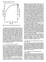
Variable acceleration:
If the acceleration is a function of
time then the area under the acceleration time curve repre-
sents the change in velocity.
If
the acceleration is a function of
displacement then the area under the acceleration distance
curve represents half the difference of the square of the
velocities (see Figure
1.4).
Curvilinear motion
is when both linear and angular motions
are present.
If a particle has a velocity
v
and an acceleration
a
then its
motion may be described
in
the following ways:
1.
Cartesian components
which represent the velocity and
acceleration along two mutually perpendicular axes

x
and
y
(see Figure 1.5(a)):
a
t
dv
a
=
-
oradt=dv
dt
Area a.dt
=
vz
-
v,
a
a=
*.
dv
dt dx
dv
a=v
-
dx
2
X
or adx
=

vdv
X
Figure
1.4
Dynamics
of
rigid bodies
1/7
Figure
1.5
I
Normal
vx
=
v
cos
6,
vy
=
v
sin
8,
ax
=
a
cos
+,
ay
:=
a

sin
4
Normal and tangential components:
see Figure
1.5(b):
v,
=
v =
r6
=
ro,
vn
=
0
a,
=
rO,
+
ra
+
io,
a,
=
vB
=
rw'
2.
E
is
on

the
link
F
is
on
the slider
3.
Pobzr
coordinates:
see Figure 1.5(c):
vr
=
i,
"8
=
~8
a,
=
i
-
rV,
as
=
4
+
2i.i
1.3.3 Circular motion
Circular motion is a special case
of
curvilinear motion in which

the radius of rotation remains constant.
In
this case there is an
acceleration towards the cente of
0%.
This gives rise to a force
towards the centre known as the
centripetal force.
This force
is
reacted to by what is called the
centrifugal reaction.
Veloc,ity and acceleration in mechanisms:
A
simple approach
to
deter:mine the velocity and acceleration of a mechanism at a
point in time
is
to
draw velocity and acceleration vector
diagrams.
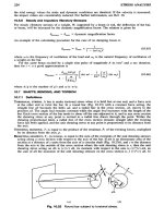
Velocities:
If
in a rigid link
AB
of
length
1
the end

A
is
moving with
a
different velocity to the end
B,
then the velocity
of
A
relative
to
B
is in a direction perpendicular
to
AB
(see
Figure
1.6).
When a block slides on a rotating link the velocity is made
up
of
two components, one being the velocity of the block
relative to the link and the other the velocity
of
the link.
Accelerations:
If
the link has an angular acceleration
01
then

there will be two components
of
acceleration in the diagram, a
tangential component
cul
and a centripetal component of
magnitude
w21
acting towards
A.
When a block §!ides
on
a rotating link the total acceleration
is composed
of
four parts: first; the centripetal acceleration
towards
0
of
magnitude
w21;
second, the tangential accelera-
tion
al;
third, the accelerarion
of
the block relative to the link;
fourth, a tangential acceleration of magnitude
2vw
known as

Coriolis acceleration. The direction
of
Coriolis acceleration is
determined
by
rotating the sliding velocity vector through
90"
in
the diirection
of
the
link
angular velocity
w.
1.3.4
1.3.4.1
xyz
is a moving coordinate system, with
its
origin at
0
which
has a position vector
R,
a translational velocity vector
R
and
an
angular velocity vector
w

relative to a fixed coordinate
system
XYZ,
origin at
0'.
Then the motion of a point
P
whose
position vector relative to
0
is
p
and relative to
0'
is
r
is given
by the following equations (see Figure
1.7):
Linear
and angular motion in three dimensions
Motion
of
a
particle in
a
moving coordinate system
a
d
fl

Figure
1.6
r
=
1
+
pr
+
w x
p
r
=
R
+
w
x
p
+
w
x
(w
x
p)
+
2w
x
p,
+
pr
where

pr
is the velocity of the point
P
relative to the moving
system
xyz
and
w
X
p
is the vector product
of
w
and
p:
where
pr
is the acceleration
of
the point
P
relative
to
the
moving system. Thus
r
is the sum
of:
1.
The relative velocity

ir;
2.
3.
and
r
is the sum
of:
1.
The relative acceleration
Br;
2.
3.
4.
5.
The absolute velocity
R
of the moving origin
0;
The velocity
w
x
p
due to the angular velocity
of
the
moving axes
xyz.
The absolute acceleration
R
of

the moving origin
0;
The tangential acceleration
w
x
p
due
to
the angular
acceleration
of
the moving axes
xyz;
The centripetal acceleration
w
X
(w
x
p)
due
to
the
angular velocity
of
the moving axes
xyz;
Coriolis component acceleration
26.1
X
pr

due
to
the inter-
action of coordinate angular velocity and relative velocity.
1/8
Mechanical engineering principles
1.3.6
Balancing
of
rotating
masses
't
1.3.6.1
Single out-of-balance
mass
P
Y
Figure
1.7
V
Precession axis
Spin
5%
axis
One mass
(m)
at a distance
r
from the centre of rotation and
rotating at a constant angular velocity

w
produces a force
mw2r.
This can be balanced
by
a mass
M
placed diametrically
opposite at a distance
R,
such that
MR
=
mr.
t
v
1.3.6.2 Several out-of-balance masses in one transverse
plane
If a number of masses
(ml, m2,
.
. .
)
are at radii
(II,
r2,
.
.
.
)

and angles
(el,
e,,
. .
.
)
(see Figure
1.9)
then the balancing
mass
M
must be placed at a radius
R
such that
MR
is
the vector
sum of all the
mr
terms.
1.3.6.3 Masses in different transverse planes
If
the balancing mass in the case of a single out-of-balance
mass were placed in a different plane then the centrifugal force
would be balanced. This is known as
static balancing.
However, the moment of the balancing mass about the
't
axis
X

Figure
1.8
In
all the vector notation a right-handed set of coordinate axes
and the right-hand screw rule is used.
CFx
=
Crnw2r
sin
0
=
0
CFy
=
Crnw2r
cos
0
=
0
Figure
1.9
1.3.4.2 Gyroscopic efjects
Consider a rotor which spins about its geometric axis (see
Figure
1.8)
with an angular velocity
w.
Then two forces
F
acting

on
the axle to form a torque
T,
whose vector is along
the
x
axis, will produce a rotation about the
y
axis. This is
known as precession, and it has an angular velocity
0.
It
is
also
the case that
if
the rotor is precessed then a torque Twill be
produced, where
T
is given by
T
=
IXxwf2.
When this is
observed it is the effect
of
gyroscopic reaction torque that is
seen, which is in the opposite direction to the gyroscopic
torq~e.~
1.3.5

Balancing
In any rotational or reciprocating machine where accelerations
are present, unbalanced forces can lead
to
high stresses and
vibrations. The principle
of
balancing is such that by the
addition
of
extra masses to the system the out-of-balance
forces may be reduced or eliminated.
CFx
=
Zrnw2r
sin
0
=
0
and
ZFy
=
Zrnw2r
cos
0
=
0
as
in
the previous case,

also
ZM~
=
Zrnw2r
sin
e
.
a
=
o
zMy
=
Crnw2r
cos
e
.a
=
0
Figure
1.10
Vibrations
119
1.4
Vibrations
1.4.1
Single-degree-of-freedom systems
The term degrees of freedom in an elastic vibrating system
is
the number
of

parameters required
to
define the configuration
of the system. To analyse a vibrating system a mathematical
model is constructed, which consists of springs and masses for
linear vibrations. The type of analysis then used depends on
the complexity of the model.
Rayleigh’s method: Rayleigh showed that if a reasonable
deflection curve
is
assumed for a vibrating system, then by
considering the kinetic and potential energies” an estimate
to
the first natural frequency could be found.
If
an inaccurate
curve is used then the system is subject
to
constraints
to
vibrate it in this unreal form, and this implies extra stiffness
such that the natural frequency found will always be high.
If
the exact deflection curve
is
used then the nataral frequency
will be exact.
original plane would lead
to
what

is
known as dynamic
unbalan,ce.
To overcome this, the vector sum
of
all the moments about
the reference plane must also be zero.
In
general, this requires
two
masses placed in convenient planes (see Figure 1.10).
1.3.6.4
Balancing
of
reciprocating masses in single-cylinder
machines
The accderation
of
a piston-as shown in Figure 1.11 may be
represented by the equation>
i
=
-w’r[cos
B
+
(1in)cos
28
+
(Mn)
(cos

26
-
cos 40)
+
,
.
. .
];k
where
n
=
lir. If
n
is large then the equation may be
simplified and the force given by
F
=
mi
=
-mw2r[cos
B
+
(1in)cos
201
The term mw’rcos
9
is
known as the primary force and
(lln)mw2rcos
20

as the secondary force. Partial primary
balance
is
achieved in a single-cylinder machine by an extra
mass
M
at a radius
R
rotating at the crankshaft speed. Partial
secondary balance could be achieved by a mass rotating at
2w.
As
this is not practical this
is
not attempted. When partial
primary balance is attempted a transverse component
Mw’Rsin
B
is
introduced. The values of
M
and
R
are chosen to
produce a compromise between the reciprocating and the
transvense components.
1.3.6.5
When considering multi-cylinder machines account must be
taken
of

the force produced by each cylinder and the moment
of
that force about some datum. The conditions for primary
balance are
F
=
Smw2r cos
B
=
0,
M
=
Smw’rcos
o
.
a
=
O
where a is the distance of the reciprocating mass
rn
from the
datum plane.
In general, the cranks in multi-cylinder engines are arranged
to
assist primary balance.
If
primary balance is not complete
then extra masses may be added to the crankshaft but these
will introduce an unbalanced transverse component. The
conditions for secondary balance are

F
=
Zm,w2(r/n) cos 20
=
&~(2w)~(r/4n) cos 20
=
o
and
M
=
Sm(2~)~(r/4n) cos 20
.
a
=
0
The addition
of
extra masses to give secondary balance is not
attempted in practical situations.
Balancing of reciprocating masses in multi-cylinder
machines
Y>
W
I
Mass
m
\
1R
\
LM

Figure
1
:I
1
*
This equation forms
an
infinite series in which higher terms are
small and they may
be
ignored
for
practical situations.
1.4.1.1
Transverse vibration of beams
Consider a beam of length
(I),
weight per unit length
(w),
modulus (E) and moment
of
inertia
(I).
Then
its
equation
of
motion is given by
d4Y
EI

-
-
ww2y/g
=
0
dx4
where
o
is the natural frequency. The general solution of this
equation is given by
y
=
A
cos
px
+
B sin
px
+
C
cosh
px
+
D
sinh
px
where
p”
=
ww2igEI.

The four constants of integration
A,
B,
C
and
D
are
determined by four independent end conditions.
In
the solu-
tion trigonometrical identities are formed in
p
which may be
solved graphically, and each solution corresponds to a natural
frequency of vibration. Table
1.3
shows the solutions and
frequencies
for
standard beams.6
Dunkerley’s empirical method is used for beams with mul-
tiple loads.
In
this method the natural frequency
vi)
is found
due to just one of the loads, the rest being ignored.
This
is
repeated for each load in turn and then the naturai frequency

of vibration of the beam due to its weight alone
is
found
(fo).
*
Consider the equation
of
motion
for
an
undamped system (Figure
1.13):
dzx
d?
rn +lur=O
but
Therefore equation
(1.4)
becomes
Integrating gives
krn
($)’+’,?
2
=
Constant
the term &(dx/dt)* represents the kinetic energy and
&xz
the
potential energy.
1/10

Mechanical engineering principles
Table
1.3
End conditions Trig. equation Solutions
PI1
P21
P31
x
=
0,
y
=
0,
y‘
=
0
COS
pl
.
cash
01
=
1
4.730 7.853 10.966
x
=
1,
y
=
0,

y‘
=
0
x
=
0,
y
=
0,
y‘
=
0
COS
pl
.
cash
pl
=
-1
1.875 4.694 7.855
x
=
1,
y“
=
0,
y”’
=
0
x

=
0,
y
=
0,
y”
=
0
sin
Pl
=
0
3.142 6.283 9.425
+
-
x=l,y=O,y”=O
5
x=l,y=O,y”=O
x
=
0,
y
=
0,
y’
=
0
tan
Pl
=

tanh
Pl
3.927 7.069
10.210
Then the natural frequency of vibration
of
the complete
system
U,
is given by
11111
1
-
+-+-+-+
_-_
f2
f;
f?
f:
fS
fi
(see reference
7
for a more detailed explanation).
Whirling of shafts:
If
the speed
of
a shaft or rotor is slowly
increased from rest there will be a speed where the deflection

increases suddenly. This phenomenon is known as whirling.
Consider a shaft with a rotor of mass
m
such that the centre of
gravity
is
eccentric by an amount
e.
If
the shaft now rotates at
an angular velocity
w
then the shaft will deflect by an amount
y
due to the centrifugal reaction (see Figure
1.12).
Then
mw2(y
+
e)
=
ky
where
k
is the stiffness
of
the shaft. Therefore
e
=
(k/mw*

-1)
When
(k/mw2)
=
1, y
is
then infinite and the shaft is said to be
at its critical whirling speed
wc.
At any other angular velocity
w
the deflection
y
is given by
When
w
<
w,,
y
is the same sign as
e
and as
w
increases
towards
wc
the deflection theoretically approaches infinity.
When
w
>

w,,
y
is opposite in sign to
e
and will eventually
tend to
-e.
This is a desirable running condition with the
centre
of
gravity
of
the rotor mass on the static deflection
curve. Care must be taken not to increase
w
too high as
w
might start to approach one
of
the higher modes of vibration.8
Torsional vibrations:
The following section deals with trans-
verse vibrating systems with displacements
x
and masses
m.
The same equations may be used for torsional vibrating
systems by replacing
x
by

8
the angular displacement and
m
by
I,
the moment
of
inertia.
1.4.1.2
Undamped
free
vibrations
The equation of motion is given by
mi!
+
kx
=
0 or
x
+
wix
=
0,
where
m
is the mass,
k
the stiffness and
w:
=

k/m,
which
is
the natural frequency
of
vibration
of
the system (see
Figure
1.13).
The solution to this equation is given by
x
=
A
sin(w,t
+
a)
Figure
1.12
where
A
and
a
are constants which depend
on
the initial
conditions. This motion is said to be
simple harmonic
with a
time period

T
=
2?r/w,.
1.4.1.3
Damped free vibrations
The equation of motion is given by
mi!
+
d
+
kx
=
0
(see
Figure
1.14),
where
c
is the viscous damping coefficient, or
x
+
(c/m).i
+
OJ;X
=
0.
The solution to this equation and the
resulting motion depends
on
the amount of damping.

If
c
>
2mw,
the system is said to be overdamped. It will respond
to a disturbance by slowly returning
to
its equilibrium posi-
Vibrations
1/11
Figure 1.13
X
Figure 1.14
X
c
>
Zrnw,
tion. The time taken
to
return to this position depends on the
degree
of
damping (see Figure 1.15(c)).
If
c
=
2mw,
the
system is said to be critically damped. In this case it will
respond

to
a
disturbance by returning to its equilibrium
position in the shortest possible time. In this case (see Figure
1.15(b))
=
e-(c/2m)r(A+Br)
where
A
and
B
are constants.
If
c
<
2mw,
the system has a
transient oscillatory motion given by
=
e-(</2m)r
[C
sin(w;
-
c2i4m2)’”t
+
cos
w:
-
~~/4m~)”~t]
where

C
and
D
are constants. The period
2.ir
‘T
=
-
(wf
-
c2/4.m2)112
(see Figure
1.15(a)).
1.4.1.4
Logarithmic decrement
A
way to determine the amount
of
damping in a system is to
measure the rate
of
decay
of
successive oscillations. This is
expressed by a term called the
logarithmic decrement
(6),
which is defined as the natural logarithm
of
the ratio

of
any
two
successive amplitudes (see Figure
1.16):
6
=
log&1/x2)
c
=
Zmw,
Figure 1.15
where
x
is given by
x
=
ecnm sin
[(J
Therefore
112
=
cr12rn
If
the amount
of
damping present
is
small compared to the
where

T
is the period
of
damped oscillation.
critical damping,
T
approximates
to
27r/w,
and then
8
=
cdmw,
1/12
Mechanical engineering principles
X
A
\
\
x1
‘\
\
.
-\
.
.
I
t
4
/

F\
\
I
.
t
4
/
/
/
/
Figure
1.16
1.4.1.5
Forced undamped vibrations
The equation
of
motion is given by (see Figure 1.17)
mx
+
kx
=
Fo
sin
wt
or
x
+
w,2
=
(Fdm)

sin
wt
The solution to this equation is
x
=
C
sin
o,t
+
D
cos
w,t
+
Fo
cos
wt/[m(w;
-
w’)]
where
w
is the frequency
of
the forced vibration. The first two
terms of the solution are the transient terms which die out,
leaving an oscillation at the forcing frequency of amplitude
Fd[m(wf
-
41
or
FO

sin
wt
Fo
sin
at
(a)
Figure
1.17
The term
wt/(w;
-
w2)
is
known
as the dynamic magnifier
and it gives the ratio of the amplitude
of
the vibration to the
static deflection under the load
Fo.
When
w
=
on
the ampli-
tude becomes infinite and resonance is said to occur.
1.4.1.6
Forced damped vibrations
The equation of motion is given by (see Figure 1.17(b))
mx

+
cx
+
kx
=
Fo
sin
ut
or
E
+
(c/m)i
+
wt
=
(Fdm)
sin
wl
The solution to this equation is in two parts: a transient part as
in the undamped case which dies away, leaving a sustained
vibration at the forcing frequency given by
FO
m
x=-
1
[(wf
-
w2)’
+
(c(~/m)’]~’~

The term
sin(ot
-
4
[(wt
-
w2)’
+
(c~/m)]~]~’~
is called the dynamic magnifier. Resonance occurs when
w
=
w,.
As
the damping is increased the value of
w
for which
resonance occurs is reduced. There is also a phase shift as
w
increases tending to a maximum
of
7~
radians. It can be seen in
Figure 1.18(a) that when the forcing frequency is high com-
pared to the natural frequency the amplitude
of
vibration is
minimized.
1.4.1.7
Forced damped vibrations due

to
reciprocating
or
rotating unbalance
Figure 1.19 shows two elastically mounted systems, (a) with
the excitation supplied by the reciprocating motion of a piston,
and
(b)
by the rotation of an unbalanced rotor.
In
each case
the equation
of
motion is given by
(M
-
m)i
+
ci
+
kx
=
(mew’)
sin
wt
The solution of this equation is a sinusoid whose amplitude,
X,
is given by
X= mewL
V[(K

-
MJ)2
+
(cw)2]
In representing this information graphically it is convenient to
plot
MXlme
against
wlw,
for various levels of damping (see
Figure l.20(a)). From this figure it can be seen that for small
values of
w
the displacement is small, and as
w
is increased the
displacement reaches a maximum when
w
is slightly greater
than
w,.
As
w
is further increased the displacement tends to a
constant value such that the centre
of
gravity
of
the total mass
M

remains stationary. Figure 1.20(b) shows how the phase
angle varies with frequency.
1.4.1.8
Forced damped vibration due
to
seismic excitation
If
a system as shown in Figure 1.21 has a sinusoidal displace-
ment applied to its base of amplitude,
y,
then the equation
of
motion becomes
mx
+
ci
+
kx
=
ky
+
cy
The solution
of
this equation yields
’=
Y
J[(k-
mw’)’
+

(cw)’
where
x
is the ampiitude of motion of the system.
1
k2
+
(cw)’
Vibrations
1/13
No
damping
I
Moderate damping
Figure
1.18
1
.o
2.0
3.0
Frequency ratio
(w/w,)
(a)
/
No
damping
Critical damping
1
2
3

4
Frequency ratio
(dun)
(b)
I
I
M
I

\Cri?ical
damping
0
1
.o
2.0
3.0
4.0
Frequency ratio
(dun)
(2)
180"
(u
-
m
m
H
90"
r
Q
0

Figure
1.20
Moderate damping
1.0
2.0
3.0
4.0
Frequency ratio
(w/w,)
(b)
m
Figure
1.19
Figure
1.21
1/14
Mechanical engineering principles
When this information is plotted as in Figure 1.22 it can be
seen that for very small values
of
w
the output amplitude Xis
equal to the input amplitude
Y.
As
w
is increased towards
w,
the output reaches a maximum. When
w

=
g2
w,
the curves
intersect and the effect
of
damping is reversed.
The curves in Figure 1.22 may also be used to determine the
amount of sinusoidal force transmitted through the springs
and dampers to the supports, Le. the axis
(X/Y)
may be
replaced by
(F,IFo)
where
Fo
is the amplitude of applied force
and
Ft
is the amplitude of force transmitted.
1.4.2
Multi-degree-of-freedom
systems
1.4.2.1
Normal mode
vibration
The fundamental techniques used in modelling multi-degree-
of-freedom systems may be demonstrated by considering a
simple two-degree-of-freedom system as shown in Figure 1.23.
The equations of motion for this system are given by

mf1
+
(kl
+
k2)xl
-
kzxz
=
0
m2Xz
+
(k3
+
k2)x2
-
kzxl
=
0
or in matrix form:
L
0
1
.o
0
d
////
//
/
/
///

///////A
Figure
1.23
Assuming the motion
of
every point in the system to be
harmonic then the solutions will take the form
x1
=
AI
sin
ot
x2
=
Az
sin
ut
where
A1
and
A2
are the amplitudes of the respective displace-
ments. By substituting the values of
XI,
x2,
XI
and
x2
into the
original equations the values of the natural frequencies of

vibration may be found along with the appropriate mode
shapes. This is a slow and tedious process, especially for
systems with large numbers of degrees of freedom, and is best
performed by a computer program.
1.4.2.2
The
Holtzer method
When only one degree
of
freedom is associated with each mass
in a multi-mass system then a solution can be found by
proceeding numerically from one end of the system to the
other.
If
the system is being forced to vibrate at a particular
frequency then there must be a specific external force
to
produce this situation. A frequency and a unit deflection is
assumed at the first mass and from this the inertia and spring
forces are calculated at the second mass. This process is
repeated until the force at the final mass is found.
If
this force
is zero then the assumed frequency is a natural frequency.
Computer analysis is most suitable for solving problems of this
type.
Consider several springs and masses as shown in Figure
1.24. Then with a unit deflection at the mass
ml
and an

assumed frequency
w
there will be an inertia force of
mlw2
acting on the spring with stiffness
kl.
This causes a deflection
of
mlw2/kl,
but if
m2
has moved a distance
x2
then
mlw2/
kl
=
1
-
x2
or
x2
=
1
-
mlwz/kl.
The inertia force acting due
to
m2
is

m2w2x2,
thus iving the total force acting on the spring
Critical
1.0
d2
2.0
3.0
of
stiffness
k2
as
fmlw
4
+
m202xz}/kz.
Hence the displacement
Frequency ratio
(w/w,)
(a)
0
Low
damping
Moderate
1800w
1234 damping
Frequency ratio
(w/w,)
(
b)
~~~

at
xj
can be found and the procedure repeated. The external
force acting on the final mass is then given by
2
m,w2x1
i=1
If
this force is zero then the assumed frequency is a natural
one.
Figure
1.22
Figure 1.24