Optimal condition based maintenance via a mobile
Bạn đang xem bản rút gọn của tài liệu. Xem và tải ngay bản đầy đủ của tài liệu tại đây (3.79 MB, 26 trang )
<span class="text_page_counter">Trang 1</span><div class="page_container" data-page="1">
INFORMS is located in Maryland, USA
Shadi Sanoubar, Bram de Jonge, Lisa M. Maillart, Oleg A. Prokopyev
<b>To cite this article:</b>
Shadi Sanoubar, Bram de Jonge, Lisa M. Maillart, Oleg A. Prokopyev (2023) Optimal Condition-Based Maintenance via a Mobile Maintenance Resource. Transportation Science 57(6):1646-1670. terms and conditions of use: article may be used only for the purposes of research, teaching, and/or private study. Commercial use or systematic downloading (by robots or other automatic processes) is prohibited without explicit Publisher approval, unless otherwise noted. For more information, contact
The Publisher does not warrant or guarantee the article’s accuracy, completeness, merchantability, fitness for a particular purpose, or non-infringement. Descriptions of, or references to, products or publications, or inclusion of an advertisement in this article, neither constitutes nor implies a guarantee, endorsement, or support of claims made of that product, publication, or service.
Copyright © 2023, INFORMS
<b>Please scroll down for article—it is on subsequent pages</b>
With 12,500 members from nearly 90 countries, INFORMS is the largest international association of operations research (O.R.) and analytics professionals and students. INFORMS provides unique networking and learning opportunities for individual professionals, and organizations of all types and sizes, to better understand and use O.R. and analytics tools and methods to transform strategic visions and achieve better outcomes.
For more information on INFORMS, its publications, membership, or meetings visit
</div><span class="text_page_counter">Trang 2</span><div class="page_container" data-page="2"><b>Optimal Condition-Based Maintenance via a Mobile Maintenance Resource</b>
<b><small>Shadi Sanoubar,</small><sup>a </sup><small>Bram de Jonge,</small><sup>b </sup><small>Lisa M. Maillart,</small><sup>a,</sup><small>* Oleg A. Prokopyev</small><sup>a,c </sup></b>
<small>Department of Industrial Engineering, University of Pittsburgh, Pittsburgh, Pennsylvania 15261; </small><b><sup>b</sup></b><small>Department of Operations, Faculty of Economics and Business, University of Groningen, 9747 AE Groningen, Netherlands; </small><b><sup>c</sup></b><small>Department of Business Administration, University of Zurich, CH-8032 Zurich, Switzerland </small>
<small>*Corresponding author </small>
<b><small>Contact: </small></b><small>, , </small>
<small>, , </small>
<b><small>Abstract. </small></b><i>We consider the problem of performing condition-based maintenance on a set of </i>
<i>geographically distributed assets via a single maintenance resource that travels between the </i>
assets’ locations. That is, we dynamically determine the optimal positioning of the mainte-nance resource and the optimal timing of condition-based maintemainte-nance interventions that the maintenance resource performs. These decisions are made as a function of the condi-tions of the assets and the current location of the maintenance resource to minimize total expected costs, which include downtime, travel, and maintenance expenses. This holistic approach enables us to study unique trade-offs, namely, maintaining an asset early if the
<i>maintenance resource is currently close by, or alternatively, optimally repositioning the </i>
<i>maintenance resource or having it idle in key locations in anticipation of asset deterioration. </i>
We model the location of the maintenance resource and assets using a graph representation and the assets’ deterioration process as a discrete-time Markov chain. We formulate a Mar-kov decision process to obtain the optimal policy for the maintenance resource (i.e., where to travel, idle, or repair). We explore the properties of the optimal policies (analytically and numerically) and how they are affected by the graph structure. Finally, we develop and analyze some implementation-friendly heuristic policies.
<b><small>Funding: This research was supported by Pitt Momentum Fund Award (3463) and NSF [Grant CMMI- </small></b>
<small>2002681]. </small>
<b><small>Supplemental Material: The online appendix is available at </small></b><small> </small>
<b><small>Keywords:condition-based maintenance</small></b><small>•</small><b><small>proximal maintenance</small></b><small>•</small><b><small>dynamic positioning</small></b><small>•</small><b><small>Markov decision process</small></b><small>•</small><b><small>network</small></b><small>•</small>
<b><small>node centrality</small></b>
<b>1. Introduction</b>
Recent advances in sensor technologies and remote mon-itoring tools have facilitated real-time tracking of asset health parameters that enable the implementation of condition-based maintenance (CBM) strategies. A CBM strategy prescribes maintenance activities dynamically/ adaptively over time based on condition monitoring information, resulting in more cost-effective mainte-nance plans compared with traditional approaches. The global condition monitoring market size is projected to grow from $2.8 billion in 2022 to $4.0 billion by 2028, with North America as a key market for these technolo-gies (MarketsandMarkets 2022). This growth in the condition-monitoring market is also fueled by recent shifts in many industries toward automation, spurred in part by the “great resignation,” which resulted in an increase of up to 37% in robotic orders of North American companies in 2021 compared with 2020 (Morris 2021). Numerous industries, especially those with capital-intensive invest-ments, have recently adopted CBM strategies. Some
examples include transportation networks, marine tech-nologies, aerospace and defense industries, oil and gas pipelines, and IT infrastructures (Telford, Mazhar, and Howard 2011; Prajapati, Bechtel, and Ganesan 2012; Xu et al. 2014; M´erigaud and Ringwood 2016).
Common characteristics shared by many of these
<i>indus-try applications include a set of geographically dispersed assets that must be maintained by a limited number of maintenance resources. In such settings, the maintenance resources may </i>
be positioned between the asset locations and travel to the assets to maintain (e.g., repair or replace) them.
The maintenance resources in these settings may be human crews, heavy equipment and materials, or, increasingly, self-propelled maintenance robots. Con-sider, for example, railway transportation, in which crews and equipment are positioned in anticipation of performing many types of activities to maintain its infra-structure composed of tracks, bridges, tunnels, signals, and other equipment (Hodge et al. 2015). In terms of inspection and maintenance robots, it is worth noting
</div><span class="text_page_counter">Trang 3</span><div class="page_container" data-page="3">that their market size is projected to grow from $1.7 billion in 2020 to $3.5 billion by 2028 (Mueller 2019, Data Insights Partner 2021). Example applications of these robots include customer fulfillment centers, sub-sea installations and technologies, water pipelines, and computer server centers (Ahrary, Nassiraei, and Ishi-kawa 2007; Liljebăack and Mills 2017; Boyle 2018; Asfour et al. 2019).
In all of these applications, an effective mainte-nance plan requires the integrated optimization of two
<i>decision-making processes, namely, the timing of mainte-nance interventions and the repositioning of maintemainte-nance resources (e.g., specialized equipment, human crews, and robots) using the assets’ condition information. This </i>
complex decision space gives rise to unique and, as of yet, not well-understood trade-offs. For example, when maintaining a set of geographically dispersed condition- monitored assets, it may be optimal to maintain an asset earlier than it would be for that asset in isolation if a maintenance resource is currently “sufficiently close” to the location of the asset. Or, based on current condition
<i>information, it may be optimal to reposition maintenance resources or have them idle in key locations in </i>
anticipa-tion of asset deterioraanticipa-tion that would prompt a future maintenance action.
<b>1.1. Problem Definition</b>
Consider a set of identical, geographically distributed assets that degrade stochastically over time and may fail without proper intervention. Failures do not man-date immediate maintenance but do incur downtime costs. A single maintenance resource is tasked with traveling among and maintaining these assets. We model the asset deterioration process as a completely observable discrete-time Markov chain and the location of the maintenance resource and assets using a graph (network). In this graph, nodes represent possible geo-graphical locations for the maintenance resource, which include both auxiliary and asset locations. Traversing the auxiliary locations allows the maintenance resource to reach asset locations. The maintenance resource may also idle at the auxiliary or asset locations at any time. Edges represent links between nodes along which the maintenance resource may travel. We assume that assets are not co-located, and hence, the maintenance resource travels between asset nodes to carry out re-pairs, which restore the assets to as-good-as-new.
<i>We seek to (i) dynamically obtain the optimal actions </i>
(repair, reposition, idle) for the maintenance resource as a function of the conditions of the assets and the cur-rent location of the resource to minimize total expected discounted costs that include downtime, travel, and
<i>maintenance expenses; (ii) study the structural proper-ties of the optimal policies; (iii) provide insights on how </i>
current and future locations of the resource can be exploited to perform proximal maintenance, and how
the maintenance resource can be strategically
<i>reposi-tioned in anticipation of maintenance needs; (iv) </i>
ex-plore how the graph structure affects positioning and
<i>maintenance decisions; and (v) design implementation- </i>
friendly heuristic policies.
<b>1.2. Literature Review and Our Contributions</b>
The majority of studies on condition-based mainte-nance focus on adaptively determining when to per-form maintenance as a function of the condition of a single asset or multiple co-located assets with eco-nomic dependencies; we refer the reader to de Jonge and Scarf (2020) and Alaswad and Xiang (2017) for a review. To the best of our knowledge, the only exist-ing work on condition-based maintenance for dis-persed assets is that in Havinga and de Jonge (2020). In their work, the assets are dispersed on a cycle graph and are visited in a fixed order by a maintenance resource, and hence, no decisions are made on how to dynamically reposition the resource. Our modeling framework, on the other hand, generalizes the graph configuration and addresses both the timing of main-tenance interventions and the dynamic repositioning of the maintenance resource. A recent survey points out that condition-based maintenance of geographi-cally dispersed assets is an open research direction (de Jonge and Scarf 2020).
Other related studies have considered preventive maintenance for geographically dispersed assets, but in the context of “time-based maintenance.” In time- based maintenance, maintenance interventions are pre-scribed based on the assets’ lifetime (age) distributions in the absence of real-time condition information (see de Jonge, Teunter, and Tinga 2017for a comparison of time-based and condition-based maintenance). These studies include Goel and Meisel (2013), L ´opez-Santana et al. (2016), Schrotenboer et al. (2018), Rashidnejad, Ebrahimnejad, and Safari (2018), Nguyen et al. (2019), and Fan et al. (2019), who consider deterministic settings where a set of maintenance tasks are predefined or scheduled based on the assets’ ages and are carried out by multiple resources. Similarly, Camci (2014, 2015) determined optimal routes a priori that are updated once an asset fails. In Jia and Zhang (2019) and Chen et al. (2017), asset locations are modeled in a flow net-work, where asset failures on graph nodes can inter-rupt the flow of material in the network; but again, lifetime distributions are used to make maintenance decisions a priori. Other studies have considered rout-ing mobile assets to fixed maintenance facilities in which maintenance schedules are predefined or deter-mined based on a number of operating hours (Feo and Bard 1989, Talluri 1998, Safaei and Jardine 2018). Unlike this body of literature, in our problem, mainte-nance actions and movements of the maintemainte-nance resource are dynamically prescribed in response to
</div><span class="text_page_counter">Trang 4</span><div class="page_container" data-page="4">changes in the assets’ conditions, enabling mainte-nance planners to exploit the cost-saving benefits of condition monitoring.
Our research also has loose connections with the dynamic traveling repairman problem (Bertsimas and Van Ryzin 1991, 1993a,b), the medical unit dispatching literature (Maxwell et al. 2010, 2014; Alanis, Ingolfsson, and Kolfal 2013; Keneally, Robbins, and Lunday 2016), and dynamic repositioning problems for general applica-tions (Berman 1981a,b; Drent, Keizer, and van Houtum 2020). Thomas (2007) studied optimal waiting strategies when anticipating service requests from multiple cus-tomer locations. Other studies have considered dynamic vehicle-routing problems in which some of the customer demands are known a priori whereas others are dynamic (Larsen, Madsen, and Solomon 2002, 2004; Bent and Van Hentenryck 2004). In these studies, demands arrive sto-chastically (either in some Euclidean space or a general network) and can be viewed in a maintenance context as failed assets that (unlike our assets) require immediate maintenance. Our work, however, focuses on applica-tions with condition-monitoring technologies put in place to enable maintenance planners to maintain assets before failure. Hence, the models in this body of literature can-not adequately address the trade-offs in our maintenance setting.
Finally, another somewhat relevant body of litera-ture is that on the inventory routing problem, in which a supplier decides each period how much to deliver to each customer and how to assign trucks/routes (see Coelho, Cordeau, and Laporte 2014 for a review). In these studies, inventory is often distributed from a depot to a set of customers using a fleet of vehicles with limited capacity (Kleywegt, Nori, and Savelsbergh 2002, 2004; Campbell and Savelsbergh 2004) or is redis-tributed between different stations as in a bike-sharing system (Brinkmann, Ulmer, and Mattfeld 2019, 2020). In relation to our problem, customer (or station) in-ventory levels can be viewed as asset deterioration con-ditions and replenishment decisions as maintenance interventions. That said, in inventory routing, demand is assumed to be either deterministic or independently and identically distributed at each customer; in our set-ting, the probability of transitioning to a new deteriora-tion condideteriora-tion depends on the current deterioradeteriora-tion condition. Our model also allows for transitioning to better conditions even in the absence of maintenance. Moreover, similar to the vehicle-routing literature, these studies identify only delivery routes that must start and end at a depot and do not allow idling. Lastly, the cost structures in these problems differ from ours in that they may include inventory holding costs, delivery rewards, or shortage penalties.
Table 1summarizes the most relevant literature and highlights our contributions. The first column lists the attributes of interest. For example, the second attribute
labeled as “Allow maintenance before failure” signifies whether maintenance is allowed at failure only or if maintenance is allowed before failure as well. Similarly, the third and fourth attributes determine whether main-tenance or positioning decisions are dynamic or pre-planned. The last attribute indicates the methodology used (MDP, QT and DO stand for Markov decision pro-cesses, Queueing Theory, and Deterministic Optimiza-tion respectively). Notice that our work is the first to jointly address optimal condition-based maintenance and dynamic positioning of a maintenance resource. Table 1 also identifies potential future directions, for instance, considering condition-based maintenance for dispersed assets with partially observable conditions.
The remainder of the paper is structured as follows. Section 2formulates a Markov decision process model to obtain the optimal actions of the maintenance re-source. Section 3establishes structural properties of the optimal policy obtained from our theoretical deriva-tions. Section 4provides insights on the structure of the optimal policy obtained from numerical observations. In particular, we explore scenarios in which mainte-nance is earlier compared with a single-asset setting
<i>and introduce the concept of proximal maintenance. </i>
Moreover, we explore the use of graph centrality mea-sures to identify promising idling locations for the maintenance resource and present insights on optimal repositioning decisions. Section 5analyzes the sensitiv-ity of several metrics of interest to various parameter values (e.g., costs or transition probabilities). Section 6 provides easy-to-implement heuristic policies and ana-lyzes their performance. Finally, Section 7summarizes our findings and discusses future research directions. The appendices contain the proofs for all established results and additional numerical examples.
<b>2. Model Formulation</b>
Consider a single maintenance resource responsible for
<i>maintaining a set of n<small>M </small></i>identical assets. We use graph
<i>G � (V, E) to capture the geographical locations of the </i>
assets and possible repositioning movements between them executed by the maintenance resource. The set of
<i>nodes V consists of two disjoint subsets V<small>M </small>and V<small>T</small></i>,
<i>that is, V � V<small>M</small></i>∪<i>V<small>T </small>and V<small>M</small></i>∩<i>V<small>T</small></i>� ∅<i>. Nodes in V<small>M</small></i>� {<i>1, : : : , n<small>M</small></i>}represent the locations of the assets. Nodes
<i>in V<small>T</small></i>� {<i>l</i><small>1</small><i>, : : : , l<small>nT</small></i>}are “auxiliary” nodes that are used to model travel between the assets. The maintenance resource idles in or travels through these locations to
<i>reach asset locations. Hence, V � {1, : : : , n<small>M</small>, l</i><small>1</small><i>, : : : , l<small>nT</small></i>}. In our infinite horizon model, time is discretized, and it is assumed that the maintenance resource can traverse one graph edge per time period. For each pair of nodes
<i>b, b</i><small>′</small>∈<i>V, b ≠ b</i><small>′</small><i>, the edge (b, b</i><small>′</small>)is contained in the set of
<i>edges E if and only if it is possible to move from node b to node b</i><small>′</small>within one time period. The maintenance
</div><span class="text_page_counter">Trang 6</span><div class="page_container" data-page="6">resource can traverse the edges of the graph and may repair an asset once it is located in an asset node. Simi-lar to traversing an edge, a repair action is assumed to take one time period and restores the asset to as-good- as-new. We assume that the maintenance resource has no home base requirements and is available at all deci-sion epochs.
The assets are prone to deterioration over time, and their deterioration condition is remotely monitored and fully observed by sensors. The assets are assumed to deteriorate independently according to a discrete- time Markov chain. The deterioration conditions are
<i>denoted by 0, 1, : : : , ∆ � 1, ∆, where 0 represents the as-good-as-new condition, and ∆ < ∞ represents the </i>
failed condition in which the asset is “down.” Let K � {0, 1, : : : , ∆ � 1, ∆}. We denote the transition
<i>proba-bility matrix for the discrete-time Markov chain by P, with elements P<sub>i, j </sub></i>denoting the probability of
<i>transi-tioning to deterioration condition j from i in one time </i>
Figure 1 depicts an example of a graph with four
<i>assets (n<small>M</small></i>�4) and four possible deterioration
<i>condi-tions (∆ � 3) as well as five auxiliary nodes (n<small>T</small></i>�5). Auxiliary nodes capture travel distances and possible travel routes between assets. For instance, it takes six units of time to travel from Asset 1 to Asset 4. That is, the maintenance resource must traverse the auxiliary
<i>nodes l</i><small>1</small><i>, l</i><small>2</small><i>, : : : , l</i><small>5 </small>to reach Asset 4 when repositioning from Asset 1.
As depicted in Figure 1, we generally consider set-tings where travel durations between assets are rela-tively longer than repair times (recall that a repair action takes one unit of time). Our model is motivated by applications that arise in fulfillment centers, ware-houses and manufacturing plants, and data centers as well as recently developed satellite maintenance sys-tems (Roesler, Jaffe, and Henshaw 2017; Boyle 2018; Asfour et al. 2019). In these applications, maintenance tasks often include simple and quick fixes or compo-nent replacements. For instance, in a data center, main-tenance tasks include replacing generators, switches,
and backup batteries (Zheng et al. 2013). Thus, a human technician or a servicing robot travels long dis-tances between servers and performs quick repairs upon arrival.
Next, we formulate the components of our MDP model.
<b>2.1. State Space</b>
The state of the MDP includes the deterioration condi-tions of the assets and the location of the maintenance resource because these are the only pieces of informa-tion needed to determine the resource’s next acinforma-tion.
<i>Specifically, let x<small>i </small></i>denote the deterioration condition of
<i>asset i ∈ V<small>M </small><b>and x � (x</b></i><small>1</small><i>, : : : , x<small>nM</small></i>)be the vector of deteri-oration conditions of all the assets. Furthermore, let
<i>l ∈ V denote the current location of the maintenance </i>
<i><b>resource. The state of the MDP is then s � (x, l), and the </b></i>
<i>state space S is</i>
<i><b>S � {(x, l) : x ∈ K</b><sup>n</sup><small>M</small>, l ∈ V}:</i>
<b>2.2. Actions</b>
We consider three types of actions. When the mainte-nance resource is in an asset location, a repair may be
<i>carried out (action R); the maintenance resource may also travel to an adjacent node b (action T<small>b</small></i>), or the main-tenance resource can do nothing, that is, it is idle (action
<i>DN). When the maintenance resource is in an auxiliary </i>
node, it may either travel to an adjacent node or do
<i>nothing. The set of allowable actions, denoted by A<b><small>s</small></b></i>,
<i><b>depends on the current state s � (x, l) and is expressed </b></i>
<i><b>Let p(s</b></i><small>′</small>|<i><b>s, a) denote the probability of transitioning to </b></i>
<i><b>state s</b></i><small>′</small>� (<i><b>x</b></i><small>′</small><i>, l</i><small>′</small>)<i><b>when the current state is s and action a </b></i>
is chosen. Recall that repair actions are perfect, that is, they restore the asset to an as-good-as-new condition. If
<i>the repair action is chosen (i.e., a � R), then the only </i>
pos-sible transitions are to states in which the repaired asset
<i>is as good as new and maintenance resource location l</i><small>′</small>
<i>is the same as the current location l:</i>
On the other hand, if the do-nothing action is chosen
<i>(i.e., a � DN), then the only possible transitions are to states in which maintenance resource location l</i><small>′</small> is the
<b>Figure 1. </b>(Color online) Example of a (2,4)-Banana Graph (Sethuraman and Jesintha 2009<i>) with Four Asset Nodes (V<small>M </small></i>
� {1, 2, 3, 4}) and Five Auxiliary Nodes (V<i><small>T</small></i>� {<i>l</i><small>1</small><i>, : : : , l</i><small>5</small>})
<i><small>Notes. Each asset can be in one of four deterioration conditions (K �</small></i>
<small>{0, 1, 2, ∆ � 3}); darker asset nodes indicate worse conditions. Asset conditions are also indicated on the labels next to the assets.</small>
</div><span class="text_page_counter">Trang 7</span><div class="page_container" data-page="7"><i>same as the current location l:</i>
<i>Finally, if travel action to node b is chosen (i.e., a � T<small>b</small></i>), then the only possible transitions are to states in which
<i>maintenance resource location l</i><sup>′</sup><i>is b:</i>
Three types of costs may be incurred: repair, down-time, and travel. The cost of repairing an asset in
<i>condi-tion k ∈ K is denoted by c<small>R</small></i>(k) ≥ 0. We assume that the repair cost is nondecreasing in deterioration condition because it may be more costly to repair or replace a highly deteriorated asset compared with a healthier
<i>asset. That is, 0 ≤ c<small>R</small></i>(0) ≤ ⋯ ≤ c<i><small>R</small></i>(∆). This assumption is common in the maintenance optimization literature (Barron and Yechiali 2017, Finkelstein and Eryilmaz 2021). A per-unit downtime cost c<i><small>D</small></i>≥0 is incurred in each period by any asset that is not functioning because it is either in the failed state or undergoing repair. A
<i>travel cost c<small>T</small></i>≥0 is incurred for traversing any edge (<i>b, b</i><small>′</small>) ∈<i>E.</i>
Using the above notation, the state and action-
<i><b>dependent immediate costs r(s, a) can be expressed as</b></i>
Equation (1), for example, can be interpreted as follows.
<i><b>If the repair action is chosen in state s � ((x</b></i><small>1</small><i>, : : : , x<small>l</small>, : : : , x<small>nM</small></i>)<i>, l), then the immediate cost is the summation of asset l’s repair and downtime cost plus the downtime </i>
cost of any other failed assets. Equations (2) and (3) can be interpreted in a similar manner.
<b>2.5. Value Function</b>
The overall goal is to minimize the long-run total ex-pected discounted cost by choosing optimal actions as a
<i>function of the MDP state. Let v(s) be the expected </i>
<i><b>mini-mal discounted cost to go starting from state s � (x, l), </b></i>
and let λ ∈ [0, 1) be a discount factor. Then,
Equations (5)–(7) represent the total expected
<i><b>dis-counted cost to go starting from state s and choosing </b></i>
<i>action repair, do nothing, and travel to node b, </i>
<i><b>respec-tively. The optimal action in state s, denoted by a</b></i><small>∗</small>(<i><b>s), is </b></i>
the one that obtains the minimum on the right-hand side of Equation (4). In the remainder of this paper, we use the value iteration algorithm to compute the value func-tion in (4) and obtain the optimal acfunc-tions (Puterman 2014).
<b>3. Structural Properties</b>
For analyzing the structural properties of the value func-tion and optimal policies, we first provide the definifunc-tion of an increasing failure rate (IFR) stochastic matrix (Bar-low and Proschan 1965).
<b>Definition 1.</b> Let <sup>P</sup><sup>∆</sup><i><sub>j�k</sub>P<small>i, j </small>be nondecreasing in i for all k ∈ K. Then, matrix P has the increasing failure rate </i>
(IFR) property.
The IFR property indicates that assets deteriorate fas-ter in worse conditions (see e.g., AbdulMalak and Khar-oufeh 2018and He, Maillart, and Prokopyev 2019). The deterioration processes of many real-world applications exhibit both IFR and upper-triangular properties (Byon and Ding 2010, Abdul-Malak and Kharoufeh 2018, He et al. 2019, Hoffman et al. 2021). Upper-triangularity implies that asset conditions cannot improve in the ab-sence of maintenance interventions, but it is neither re-quired for nor implied by the IFR property.
We next show that under the IFR property, the opti-mal value function is monotonically nondecreasing in
</div><span class="text_page_counter">Trang 8</span><div class="page_container" data-page="8">each asset’s condition when all other state variables remain fixed. All proofs are provided in Appendix A.
<b>Proposition 1.</b><i>If P has the IFR property, then v((x</i><small>1</small><i>, : : : , x<small>i</small>, : : : , x<small>nM</small></i>)<i>, l) is nondecreasing in x<small>i </small>for fixed l and x<small>j</small>, j ≠ i.</i>
Using Proposition 1, we establish sufficient condi-tions for the existence of an optimal control limit for the repair action with respect to the condition of the asset that is located in the position of the maintenance resource.
<b>Theorem 1.</b><i>Consider the following two sets of conditions. (i) P has the IFR property, and c<small>R</small></i>(k) is constant for all
<i>k ∈ K; (ii) P has the IFR property, c<small>R</small></i>(<i>k) is constant for all k ∈ K \ {∆}, and c<small>R</small></i>(∆) �<i>c<small>R</small></i>(∆ �<i>1) ≤ c<small>D</small>. Under either set of conditions in (i) or (ii), if there exists a condition x</i><small>∗</small>
<i><small>i </small>such that a</i><small>∗</small>((x<small>1</small><i>, : : : , x</i><sup>∗</sup><i><sub>i</sub>, : : : , x<small>nM</small></i>)<i>, i) � R, then a</i><sup>∗</sup>((x<small>1</small><i>, : : : , x<small>i</small>, : : : , x<small>nM</small></i>)<i>, i) � R for all x<small>i</small></i>≥<i>x</i><small>∗</small>
Theorem 1implies that under mild conditions, when the maintenance resource is at an asset location, the optimal maintenance decision can be characterized by a repair threshold for that asset given the deterioration conditions of other assets. This control-limit structure is appealing because it can save computational effort and is easy to implement in practice (Puterman 2014). In Section 6, we exploit this structure in developing heu-ristic policies.
The sufficient conditions of Theorem 1 ensure a control-limit structure by ruling out repair costs that are significantly higher in worse conditions; for example,
<i>the condition c<small>R</small></i>(∆) �<i>c<small>R</small></i>(∆ �<i>1) ≤ c<small>D </small></i> ensures that the difference between the repair cost at failure and at ∆ � 1 is bounded by the downtime cost. In scenarios in which repair costs are significantly higher in more deterio-rated conditions compared with better conditions, the control-limit structure may be violated. That is, it may be optimal to repair an asset in a healthier condition but suboptimal to repair it in a relatively more deteriorated condition. In the extreme of such instances, it may be optimal to abandon assets once they reach a certain level of deterioration. See examples in Appendix B. In many of our numerical examples, we let the repair cost function take more general forms (e.g., monotone increasing) than those described in the conditions of Theorem 1. However, in these examples, the repair costs do not vary significantly between different deteri-oration conditions, and we observe that the optimal repair action follows a control-limit rule.
Next, using Proposition 1, Theorem 2establishes con-ditions under which it is suboptimal to reposition to a location with a higher total expected discounted cost-to- go value.
<b>Theorem 2.</b><i>Let P have the IFR and upper-triangular prop-erties. Consider two adjacent locations l and b, that is, (l, b)</i>
∈<i><b>E. If v(x, l) � T</b></i> (<i><b>x, l), then v(x, l) ≥ λv(x, b). Moreover, </b></i>
<i><b>consider the following two sets of conditions: (i) v(x, l) < λv </b></i>
(<i><b>x, b); (ii) cT</b>><b>0 and v(x, l) ≤ λv(x, b). If either (i) or (ii) holds, then v(x, l) < T</b><small>b</small></i>(<i><b>x, l).</b></i>
The first result in Theorem 2demonstrates that if it is optimal to reposition to a particular location, then that location has a lower long-run expected discounted cost than the current location. The second result establishes the reverse case; that is, if the long-run expected dis-counted cost of a location is less than that of an adjacent location, then it is suboptimal to reposition to that
<i><b>adja-cent location. When v(x, l) � λv(x, b), the result is </b></i>
vio-lated only if the travel cost is zero.
A direct consequence of Theorem 2is that the optimal action in a node with locally minimum value function cannot be traveling and is instead idling or repairing.
<i><b>That is, if v(x, l) < λmin</b><small>b:(l, b)∈E</small><b>v(x, b), then v(x, l) � DN </b></i>
(<i><b>x, l) for l ∈ VT and v(x, l) � min{DN (x, l), R(x, l)} for l ∈</b></i>
<i>V<small>M</small></i>. Note that the upper-triangular property implies that asset conditions cannot improve in the absence of maintenance, and thus, by Proposition 1, the value
<i>func-tion at the adjacent locafunc-tion b cannot improve in the next </i>
decision epoch. Consequently, it is suboptimal to travel
<i>from node l to b in anticipation of an improvement in the </i>
value function.
<b>4. Policy Insights</b>
In this section, we discuss interesting insights on the structure of the optimal policy based on numerical experimentation. Specifically, first in Section 4.1, we discuss the factors that prompt “early” maintenance, that is, earlier than in a setting with a single asset. Then in Section 4.2, we characterize how the vector of deteri-oration conditions affects the optimal idling and reposi-tioning decisions. Lastly, in Section 4.3, we conduct a simulation study that identifies the locations in the graph that are most used for idling under the optimal policy and examine their relationship to the graph structure. We build on these findings to design high- performance heuristic policies in Section 6.
<b>4.1. Maintenance Thresholds</b>
Recall that under the IFR property and the cost condi-tions in Theorem 1, maintenance decisions when in an asset location can be characterized by an optimal repair
<i>threshold. In the special case of a single asset with a </i>
dedicated maintenance resource, this optimal repair threshold depends only on the condition-dependent repair costs, downtime cost, and the asset’s deteriora-tion process. In our more general setting, however, the optimal thresholds are affected not only by these parameter values but also by the conditions of the other assets, the relative distances between the assets, the underlying graph structure, and the current location of the maintenance resource. These novel features add to
</div><span class="text_page_counter">Trang 9</span><div class="page_container" data-page="9">the complexity of the decision-making process pertain-ing to the maintenance decisions.
In general, when the maintenance resource is at an asset location, it is often optimal to repair an asset earlier (i.e., in a less-deteriorated condition) than it would be if maintaining only that one asset in isolation; we refer to
<i>this phenomenon as early maintenance. That is, early </i>
maintenance implies that it is optimal to maintain an asset earlier in the multi-asset setting compared with the single-asset setting under the same costs and deteriora-tion process.
We summarize our numerical observations in three important scenarios where early maintenance is optimal,
<i>namely, when (i) an asset is in a noncentral and thus unfavorable location; (ii) multiple assets are deterio-rated; and (iii) the maintenance resource capitalizes on its proximity to an asset, which we refer to as proximal maintenance. Note that proximal maintenance is </i>
some-what similar to opportunistic maintenance in that it exploits opportunities to save costs by maintaining early. However, opportunistic maintenance applies to multi-component systems and uses planned or unplanned downtime caused by one component to preventively maintain another component(s) (Ding and Tian 2012, Xia et al. 2020, Zhou and Yu 2020). Therefore, the events that trigger opportunistic and proximal maintenance are
Under these parameter values, the optimal maintenance threshold for an asset in isolation is 3 (i.e., at failure). We obtain this value simply by solving the special case of our model with a single asset node.
<b>Example 1</b> (Deteriorated Asset in a Noncentral Loca-tion). One scenario in which it is optimal to maintain an asset earlier than we would for that asset in isola-tion (i.e., earlier than the deterioraisola-tion level of 3 under these parameter values) arises when the maintenance resource is near a noncentrally located asset. Main-taining such assets early can be optimal because the maintenance resource can then reposition to more central locations; take Figure 2as an example.
Figure 2depicts three scenarios, each with one deteri-orated asset. Note that in all three scenarios, the deterio-rated asset has the same deterioration level of 2, but early maintenance is only optimal in Figure 2(a)when the deteriorated asset is Asset 1, which is located in a relatively less central location. Early intervention allows
the maintenance resource to subsequently reposition to central nodes of the graph to possibly idle in antici-pation of further deterioration of the assets. That is, although not presented in Figure 2, when all assets are as good as new and the maintenance resource is at
<i>Asset 1, the optimal action is to travel toward l</i><small>1</small>. <small>w</small>
<b>Example 2</b>(Multiple Assets are Deteriorated). Another common scenario in which optimal early maintenance occurs arises when multiple assets are deteriorated. In such scenarios, by maintaining an asset early, the maintenance resource can subsequently reposition to the location of another deteriorated asset; take Figure 3 as an example. Comparing Figures 2(c)and 3, we ob-serve that early intervention is optimal in the latter because another asset is deteriorated. <small>w</small>
<b>Example 3</b>(Proximal Maintenance). Early maintenance of an asset can also be optimal because of the proximity
<b>Figure 2. </b>(Color online) An Excerpt of the Optimal Policy for Example 1
<i><small>Notes. Only in (a) is early maintenance optimal because the </small></i>
<small>deterio-rated asset is in a noncentral location. That is, early maintenance of Asset 1 allows the maintenance resource to subsequently reposition to </small>
<i><small>l</small></i><small>1, which is more central to all assets. Icons represent optimal actions as follows: repair, travel in the indicated direction. The do-nothing action is optimal in nodes with no icon.</small>
<b>Figure 3. </b>(Color online) An Excerpt of the Optimal Policy for Example 2
<i><small>Note. Early maintenance is optimal for Asset 3 because the </small></i>
<small>mainte-nance resource can subsequently travel to Asset 2 in anticipation of its further deterioration.</small>
</div><span class="text_page_counter">Trang 10</span><div class="page_container" data-page="10">of the maintenance resource to that asset; we refer to this type of early maintenance as proximal mainte-nance. In such scenarios, it may not be optimal to travel toward a deteriorated asset either because other assets are more deteriorated or because that asset is not sufficiently deteriorated to justify the costs associ-ated with traveling toward that asset. However, if the maintenance resource is already at that asset, it may be optimal to perform early maintenance; see Figure 4 as an example where proximal maintenance is optimal for Asset 1. <small>w</small>
<b>4.2. Positioning and Deterioration Conditions</b>
<i><b>To understand how the deterioration vector x affects the </b></i>
value function and the corresponding optimal actions at
<i>different locations, we look at two scenarios: (i) when </i>
deterioration levels are different among assets, that is,
<i>unbalanced; and (ii) when deterioration levels are equal </i>
among all assets, that is, balanced.
<b>4.2.1. Unbalanced Deterioration Levels. </b>When deteri-oration conditions differ among the assets, it is often optimal to move toward the assets with higher levels of deterioration. However, such policies are not necessarily optimal in general graph structures, especially when assets are not located at equally central nodes. For instance, it may be optimal to idle or move toward less deteriorated assets if the maintenance resource is close to those locations. That is, the maintenance resource would take advantage of its proximity to these assets to
perform early maintenance or idle at these locations in anticipation of further changes in their conditions. Figure 5<i>depicts an example of such a scenario for c<small>T</small></i>�1,
<b>4.2.2. Balanced Deterioration Levels. </b>When deteriora-tion levels among the assets are balanced, our numeri-cal results suggest that under sufficiently low travel costs and healthy deterioration conditions (collectively among all assets), it is optimal to travel toward the central locations of the graph and idle in anticipation of further changes. Conversely, under sufficiently high travel costs and deterioration conditions, it is optimal to travel toward and idle in the asset locations. Figure 6illustrates this claim for a (2,4)-banana tree with four assets on the leaf nodes. Specifically, Figure 6 plots the value function and the corresponding optimal actions against each node of the graph under different (balanced) deterioration conditions and travel costs. The graph configuration and the parameter settings in Figure 6are the same as those in Figure 5, except for the travel costs.
Additionally, note that in all plots of Figure 6, the locations with locally minimum long-run expected dis-counted costs correspond to idling or repairing actions as established in Theorem 2. Also, for every optimal repositioning action, the long-run expected discounted cost of the corresponding location is larger than that of the destination location (see Theorem 2).
<b>4.3. Idling and Graph Centrality</b>
In this section, our goal is to identify the locations in the graph that are used most for idling under the optimal
<i>policy and employ graph centrality measures (Newman </i>
2018) to explore the connections between these idling locations and graph structure. We simulate the optimal actions of the maintenance resource and its movement through the graph and record the number of time units
<i>the maintenance resource (i) spends in each node or (ii) </i>
idles, that is, implements the do-nothing action, in each node. We then report the long-run average fraction of time spent (or idle time spent) at each node and
<i>visual-ize these averages as heat maps.</i>
Recall from Section 2 that, under our modeling assumptions, one unit of time elapses if the optimal action is to repair an asset, idle (do nothing), or
<i>reposi-tion to an adjacent node. For metric (i), we record the </i>
cumulative time spent repairing, idling, and traveling
<i>through each node. For metric (ii), we record only the </i>
time spent idling, which we later exploit in Section 6
<b>Figure 4. </b>(Color online) An Excerpt of the Optimal Policy for Example 3
<i><small>Notes. It is not optimal to travel toward Asset 1 in l</small></i><small>1; however, if the maintenance resource is at Asset 1, then it is optimal to perform prox-imal maintenance. Note that the maintenance on Asset 2 is not proxi-mal maintenance because it is optiproxi-mal to travel toward Asset 2.</small>
<b>Figure 5. </b>(Color online) An Excerpt of the Optimal Policy for Unbalanced Deterioration Levels and High Travel Cost
<i><small>Note. It is optimal to idle at the locations close to Assets 3 and 4 even </small></i>
<small>though Assets 1 and 2 are more deteriorated.</small>
</div><span class="text_page_counter">Trang 11</span><div class="page_container" data-page="11"><i>The heat map for metric (i) can also indicate the most </i>
frequently traversed paths on the graph. Examples of heat maps for both metrics are depicted in Figure 7(b) and (c), respectively.
<b>Example 4.</b> Assume six assets dispersed on a graph as depicted in Figure 7(a). Parameter values are ∆ � 2,
To obtain the average fraction of time spent in each node, we conduct a simulation study to trace the optimal movements of the maintenance resource for 1,100,000 units of time after a warmup period of 4,000 units of time.
In the warmup period, we do not trace the movements so that we can exclude the transient behavior. These averages are then visualized as a heat map in Figure 7(b). Similarly, the averages for time spent idling are visualized only in Figure 7(c).
The heat map in Figure 7(b)illustrates the nodes at which the maintenance resource spends most of its time. Moreover, a comparison of Figure 7(b) and (c), identifies nodes used only for traveling (i.e., those with zero value in Figure 7(c)) and thus the regions most frequently traversed under the optimal policy. Notice
<i>that the maintenance resource never visits nodes l</i><small>4</small><i>, l</i><small>5</small>,
<i>and l</i><small>8 </small>because alternative paths of the same length exist and are closer to all assets; such nodes can be eliminated.
The heat map in Figure 7(c)indicates that idling is
<i>optimal only in three nodes: Asset 4, l</i><small>3</small><i>, and l</i><small>6</small>. This observation holds across a wide range of parameter
<b>Figure 6. </b>(Color online) Each Plot Depicts the Value Function and the Corresponding Optimal Actions for Different Locations in a (2,4)-Banana Tree Graph with Assets on All Four Leaf Nodes
<i><small>Notes. Travel cost increases from left to right and (balanced) deterioration conditions from top to bottom. Under low travel costs and </small></i>
<small>deteriora-tion condideteriora-tions, it is optimal to move toward and idle in the middle locadeteriora-tions of the graph. Conversely, under high travel costs and deterioradeteriora-tion conditions, it is optimal to move closer to and idle at the asset locations. Lower travel costs also prompt earlier proximal maintenance. Note that the plots are consistent with the results established in Theorems 1and 2.</small>
</div><span class="text_page_counter">Trang 12</span><div class="page_container" data-page="12">values (not presented here). Under the optimal policy, when all assets are as good as new, the maintenance resource travels toward the closest idling node (i.e., 4,
<i>l</i><small>3</small><i>, or l</i><small>6</small>) or idles if it is already at one of these nodes. When an asset slightly deteriorates (i.e., reaches dete-rioration level 1), the maintenance resource travels toward the idling node that is closest to that asset (or idles if it is located at that node). Once an asset is suffi-ciently deteriorated (i.e., reaches deterioration level 2), the maintenance resource travels toward and main-tains that asset.
Our numerical work and the examples in this section suggest that idling nodes are affected by the graph structure and tend to be centrally positioned with respect to the asset nodes. In graph theory and network analysis, centrality is a fundamental concept to identify the most “important” nodes within a graph. Various measures have been proposed that use different defini-tions of centrality to identify such important nodes; examples include degree, Eigenvector, Katz, closeness, and betweenness centrality. These measures reflect dif-ferent aspects of connectivity and are real-valued func-tions that provide a ranking of each node with respect to the centrality measure. For instance, degree centrality is characterized by the number of links incident upon a
node; Eigenvector and Katz centralities measure the influence of a node based on connections to high- scoring nodes, closeness centrality measures how close a node is on average to other nodes, and betweenness centrality quantifies how often a node acts as a bridge on the shortest path between other nodes (Newman 2018). Next, we propose two measures inspired by closeness and betweenness centralities that we believe are well-suited measures to identify idling nodes.
We define a closeness centrality measure as C(<i>l) �</i>P <sup>1</sup>
<i><small>i∈VM</small>d<small>G</small></i>(i, l)<sup>,</sup> <sup>(8) </sup>
<i>where d<small>G</small></i>(<i>i, l) denotes the length of the shortest path between nodes i and l. Note that in the denominator of </i>
(8) we only include asset nodes in the summation of graph distances because, in our application, the mainte-nance resource is positioned and travels between assets. In a typical network science application, however, the denominator may include all nodes (Newman 2018). Equation (8) assigns larger scores to nodes that are closer to all asset locations.
Interestingly, in Example 4, idling nodes 4, l<small>3</small><i>, and l</i><small>6 </small>
have the largest closeness centrality score (i.e., 1/18)
<b>Figure 7. </b><i>(Color online) Idling is Optimal Only at Nodes 4, l</i><small>3</small><i>, and l</i><small>6</small>, Which Are the Most Central Nodes with Respect to the Closeness Centrality Measure
</div><span class="text_page_counter">Trang 13</span><div class="page_container" data-page="13">among all nodes; see Figure 7(a). This example de-monstrates the relationship between the optimal pol-icy obtained through the MDP formulation and the graph structure that connects asset nodes and that this relationship can be explained by appropriate graph centrality measures such as closeness centrality. <small>w</small>
Our numerical work also suggests that betweenness centrality together with closeness centrality can iden-tify idling locations. Example 5illustrates the relation-ship between idling locations and their closeness and betweenness centrality measures.
<b>Example 5.</b> Assume four assets dispersed on a graph as depicted in Figure 8(a). Parameter values are ∆ � 3,
We run a simulation study to trace the optimal move-ments of the maintenance resource for 1,400,000 units of time after a warmup period of 40,000 units of time. The resulting heat maps are presented in Figure 8(b)and (c).
In our application, we define betweenness centrality as
<b>Figure 8. </b><i>(Color online) Idling Is Optimal at Asset Nodes and at Auxiliary Nodes l</i><small>3</small><i>, l</i><small>18</small><i>, and l</i><small>21 </small>
<i><small>Note. Among the nodes with the largest closeness centrality score, these auxiliary nodes have the largest betweenness centrality scores.</small></i>
</div>