báo cáo phương pháptính ứng dụng trong xây dựng
Bạn đang xem bản rút gọn của tài liệu. Xem và tải ngay bản đầy đủ của tài liệu tại đây (2.18 MB, 12 trang )
<span class="text_page_counter">Trang 2</span><div class="page_container" data-page="2">
<b>Họ tên SV thực hiện báo cáo:</b>
<b>Giảng viên hướng dẫn: PGS. TS NGUYỄN HOÀI SƠN</b>
</div><span class="text_page_counter">Trang 4</span><div class="page_container" data-page="4"><b>Xây dựng giải thuật:</b>
</div><span class="text_page_counter">Trang 5</span><div class="page_container" data-page="5">(1) Input the boundary and intial conditions {do} and {dḋ } the number of time steps,
<small>o</small>and the size of the time step or increment ∆t
(2) Evaluate the initial acceleration from {d } = [M]
<small>∙∙-1</small>({F
<small>o</small>} –[K]{d })
<small>o</small>(3) Solve Eq. (16.3.8) for (d )
<small>-1</small>(4) Solve Eq. (16.3.7) for {d }
<small>1</small>(5) DO i=1, Total number of time steps (6) Solve Eq. (16.3.7) for {d }
<small>i+1</small>(7) Solve Eq. (16.3.5) for {d }
<small>i</small><sup>∙∙</sup>(8) Solve Eq. (16.3.1) for {dḋ }
<small>i</small>(9) Output the displacement {d }, velocities {d }, and accelerations {d } for a given
<small>iii</small><sup>∙∙</sup></div><span class="text_page_counter">Trang 6</span><div class="page_container" data-page="6">- Gi i {ả ·d }
<small>1</small>t i tr ng di chuy nả ọể
</div><span class="text_page_counter">Trang 7</span><div class="page_container" data-page="7">Tìm đáp ứng chuyển vị và vận tốc bằng phương pháp Newmark và sai phân trung tâm.
</div><span class="text_page_counter">Trang 8</span><div class="page_container" data-page="8">Áp dụng điều kiện biên u =0 và
<small>1</small>··u
<small>1</small>=0 và đơn giản hóa chúng:
B3: Giải d tại t=-
<small>-1</small>Δt
B4: Giải d tại t= t, sử dụng giá trị d ở bước 3
<small>1</small>Δ
<small>-1</small>B5: Với giá trị d0 đã cho và d1 đã tìm được ở bước 4, tìm d2
</div><span class="text_page_counter">Trang 11</span><div class="page_container" data-page="11">tt=0:h:tmax; % time range
xk=xk+a1*xm+a1d*xd; % effective. stiff. matrix acc=xm\p; % initial acceleration
dis=zeros(2,1); % initial displacements vel=zeros(2,1); % initial velocities t=0; % initial time
kk=0; % step counter
kmax=round(tmax/h); % how many steps for tmax % dimensions of arrays to be plotted later dis1=zeros(kmax,1);
while t<=tmax, % integate while t <= tmax
[disn,veln,accn] =VTRnewmd(beta,gama,dis,vel,acc,xm,xd,xk,p,h); kk=kk+1; % increment step counter
t=t+h; % increment time value
dis1(kk)=dis(1); dis2(kk)=dis(2); % save for plotting dis=disn; vel=veln; acc=accn; % new values for next step p1=p10*sin(ome*t); p2=p20*sin(ome*t); % excitation forces % calculate steady-state response % displacements according to (5.182) are
lab=['gamma for Newmark is ' num2str(gama)]; title(lab); xlabel('time'); ylabel('particle 2')
11
</div><span class="text_page_counter">Trang 12</span><div class="page_container" data-page="12">sgama = gama*100; str_sgama = int2str(sgama); file_name = ['V2Etwodof3a' str_sgama]; print('-deps', file_name); print('-dmeta',file_name);
function [disn,veln,accn] =VTRnewmd(beta,gama,dis,vel,acc,xm,xd,xk,p,h) % Newmark integration method
% beta, gama coefficients
% dis,vel,acc displacements, velocities, accelerations at the begining of time step % disn,veln,accn corresponding quantities at the end of time step
% xm,xd mass and damping matrices % xk effective rigidity matrix % p loading vector at the end of time step
</div>