mid term report subject artificial intelligence
Bạn đang xem bản rút gọn của tài liệu. Xem và tải ngay bản đầy đủ của tài liệu tại đây (4.24 MB, 48 trang )
<span class="text_page_counter">Trang 1</span><div class="page_container" data-page="1">
<b>VIETNAM NATIONAL UNIVERSITYVIETNAM JAPAN UNIVERSITY</b>
</div><span class="text_page_counter">Trang 2</span><div class="page_container" data-page="2">II. K-means Clustering (KNN) III. Logistic Regression
IV. Support Vector Machines (SVM)
Implementation time: December 8, 2023 - December 22, 2023 Project leader: Bui The Trung
Phone: 0373.104.304 Email: Program: Bachelor of Computer Science and Engineering
LIST OF MEMBERS PARTICIPATING IN IMPLEMENTING THE PROJECT
<b>1Bùi Thế Trung</b> Code analysis SVM, KNN. Summarize the report
<b>2Phạm Quang Anh</b> Mathematical analysis SVM, write report
<b>3Lê Hải Nam</b> Implementing Linear Regression
<b>4Phạm Minh Tuấn</b> <sub>Implementing Logistic Regression</sub> <b>5Nguyễn Duy Tùng</b> Mathematical analysis KNN, write report
</div><span class="text_page_counter">Trang 3</span><div class="page_container" data-page="3"><small>2.3.1. With algorithm python...11</small>
<small>3. Comparison two results:... 13</small>
<small>4. Conclusion...13</small>
<small>5. Recommendations... 13</small>
<b><small>CHAPTER II: K-NEAREST NEIGHBOR (KNN)...14</small></b>
<small>1. Introduction... 14</small>
<small>2. Ideas and algorithms...14</small>
<small>3. Implemented in Python and Scikit-learn Python...15</small>
<small>1.3. Logistic Regression Equation:... 23</small>
<small>1.4. Logistic regression function...24</small>
<small>2. Dataset... 24</small>
<small>3. Implemented in Python...25</small>
<small>4. Implemented in Scikit Learn... 27</small>
<small>5. Conclusion...29</small>
<b><small>CHAPTER IV: SUPPORT VECTOR MACHINE (SVM)...31</small></b>
<small>1. Introduction: Distance from a point to a hyperplane...31</small>
<small>2. SVM – Optimization problem... 32</small>
<small>3. SVM – Duality problem... 35</small>
<small>3.1. Test the Slater criterion... 35</small>
<small>3.2. Largrangian SVM problem... 36</small>
<small>3.3. Lagrange dual function... 36</small>
<small>3.4. Lagrange duality problem... 38</small>
<small>3.5. Economic zone conditions... 38</small>
<small>4. Implemented in Python and Scikit-learn Python...40</small>
<small>4.1. Implemented in Python... 40</small>
<small>4.2. Implemented in Scikit-learn Python... 42</small>
<small>4.3. Summary... 45</small>
<b><small>REFERENCES...46</small></b>
</div><span class="text_page_counter">Trang 4</span><div class="page_container" data-page="4"><b>List of tables</b>
Table 1.1 : Result predicted algorithm & Sklearn Table 1.2: Comparison between two method
<b>List of shapes</b>
Figure 1.1: The linear regression model created after using the algorithm Figure 1.2: The linear regression model created after using Sklearn library Figure 2.1: Summary result KNN using algorithm
Figure 2.2: Summary result KNN using Scikit-learn
Figure 3.1: Summary result LogisticRegression using algorithm Figure 3.2: Summary result LogisticRegression using ScikitLearn Figure 4.1.1: SVM Decision Boundary
Figure 4.2.1: SVM result
Figure 4.2.2: Confusion Matrix after using Sklearn library
</div><span class="text_page_counter">Trang 5</span><div class="page_container" data-page="5">In the increasingly complex world of data, the application of machine learning algorithms to solve real-world problems has become essential. Faced with this need, our team has decided to focus on exploring and applying four leading machine learning algorithms.
We will approach these problems in two ways. Firstly, we will implement the algorithms using mathematical analysis and defining the related functions. Secondly, we will use the Scikit-learn library to apply these algorithms. We will compare the results from both methods to gain a better understanding of the performance and efficiency of our implementations.
We hope that through the execution of this project, we will not only provide solutions for the specific problems we have chosen but also contribute to expanding the understanding of how machine learning algorithms can be applied to solve real-world problems.
</div><span class="text_page_counter">Trang 6</span><div class="page_container" data-page="6"><b>CHAPTER I: LINEAR REGRESSION</b>
<b>1. Mathematical analysis</b>- Suppose that we have a predictive function: where:
+ [w1,w2,w3,...wn] is coefficient needed optimize
+ [x1,x2,x3,...xn] is vector containing parameter to train model => The objective of the model will be to find coefficients w1, w2,
- As mentioned earlier, our goal is to find coefficients w1, w2, w3,...wn such that the error between the actual value and the predicted value is minimized.
⇔ Minimize y - y'
- Using Least Ordinary least square, suppose:
- The prediction error of a value in the prediction function is given by: - From there, we will have the loss function for all values in the model
represented as follows:
</div><span class="text_page_counter">Trang 7</span><div class="page_container" data-page="7">- => The problem now is to find the coefficients w such that the value of this loss function is minimized. Let:
+ y = [y1, y2, ... yn] + X’ = [X1, X2, X3, ... Xn] => The loss function at this point will be:
- In which ||f(x)||2 is referred to as the Euclidean Norm, defined as the sum of squares of each element of the function f(x).
- To minimize the loss function, we solve the equation by setting the derivative of the function at a certain value equal to zero.
Solve (1): - We have:
As the chain rule:
and g(w) can rewrite follow as: - The derivative of loss function is:
⇔ ⇔
Solve this linear equation we have w
</div><span class="text_page_counter">Trang 8</span><div class="page_container" data-page="8"><b>2. Dataset</b>
- I will use a dataset that explores the relationship between different marketing approaches and sales figures.
- Link dataset: Sales Prediction (Simple Linear Regression) | Kaggle - The data consists of 4 fields: TV, Radio, Newspaper, Sales. These fields
represent the proportional relationship between the amount spent on each marketing channel and the resulting product sales.
- In this project, I will use 2 variables, TV and Newspaper, to create a linear regression model. This model aims to provide the most visually descriptive representation after its implementation.
<b>2.1. Implemented in Python</b>
- After reading data from the csv file, split the dataset into two parts to train and test. In which, the test dataset accounts for 75%, and the training dataset accounts for 25%.
- X is array to save information about how much money pays for advertising on TV, Z is array to save information about how much money pays for advertising in Newspapers and Y is revenue of the production when using the two methods above.
- First, we will create the design matrix X, which contains the information for training. Then, we will compute the Pseudo-inverse matrix ( ) of X.
- Applying the formula mentioned above: we obtain w.
<b>2.2. Implemented in Scikit-learn Python</b>
- Using the LinearRegression model of Scikit-learn with two parameters is X, Y.
- In which, X represents the variable that holds the matrix containing the feature information used for training the model. In this case, X is taken
</div><span class="text_page_counter">Trang 9</span><div class="page_container" data-page="9">'Newspaper'. y stands for the variable containing the target values, which refers to the 'Sales' column in the 'advertising' DataFrame. This variable holds the values that the model tries to predict or understand the relationship with the features in the matrix X.
- After that we use model.fit() to train the model.
</div><span class="text_page_counter">Trang 12</span><div class="page_container" data-page="12">Table 1.1 : Result predicted algorithm & Sklearn
<b>2.3.1. With algorithm python</b>
Figure 1.1: The linear regression model created after using the algorithm
</div><span class="text_page_counter">Trang 13</span><div class="page_container" data-page="13">Figure 1.2: The linear regression model created after using Sklearn library
</div><span class="text_page_counter">Trang 14</span><div class="page_container" data-page="14"><b>3. Comparison two results:</b>
- The two approaches yield similar results. This indicates that the algorithmic approach is accurate and somewhat superior in terms of computation time due to the use of calculation formulas
<b>4. Conclusion</b>
- Manual Linear Regression: Offers insights into underlying mathematical operations but might be less efficient and prone to implementation errors. - Scikit-learn Linear Regression: Provides an efficient, optimized, and
user-friendly interface for linear regression with reliable performance.
<b>5. Recommendations</b>
- For educational purposes or understanding the underlying mathematics, the manual implementation can be beneficial.
- For practical applications, Scikit-learn's implementation is recommended due to its efficiency, reliability, and built-in functionalities.
</div><span class="text_page_counter">Trang 15</span><div class="page_container" data-page="15"><b>CHAPTER II: K-NEAREST NEIGHBOR (KNN)</b>
<b>1. Introduction</b>K-Nearest Neighbours is one of the most basic yet essential classification algorithms in Machine Learning. It belongs to the supervised learning domain and finds intense application in pattern recognition, data mining, and intrusion detection.
It is widely disposable in real-life scenarios since it is non-parametric, meaning, it does not make any underlying assumptions about the distribution of data (as opposed to other algorithms such as GMM, which assume a Gaussian distribution of the given data). We are given some prior data (also called training data), which classifies coordinates into groups identified by an attribute.
<b>2. Ideas and algorithms</b>
Idea: The main idea of the k-NN algorithm is to predict the label of a new data point (point a) based on the closest labeled data points to it.
</div><span class="text_page_counter">Trang 16</span><div class="page_container" data-page="16"><b>Step 1: Choose quantity k</b>
We will choose a positive odd integer k , the number of nearest neighbors that the algorithm will consider to make predictions. The value of k can affect the accuracy of the model.
<b>Step 2: Measure the distance</b>
One of the most commonly used distance calculations in the KNN algorithm is the Euclidean distance; You can also use other distance calculations such as Manhattan or Minkowski
Euclidean distance: Suppose there exists a point a with coordinates ( ) and the given points have coordinates ( ). We
<b>Step 3: Find the k nearest neighbors</b>
After measuring the distance of point a to the given points, we will be able to find out which k nearest neighbors to point a are.
<b>Step 4: Make predictions</b>
Once we have the k nearest neighbors to point a, we can determine the class of the new point based on the percentage of neighbors belonging to each class.
<b>3. Implemented in Python and Scikit-learn Python3.1. Implemented in Python</b>
Data Loading and Preprocessing:
</div><span class="text_page_counter">Trang 17</span><div class="page_container" data-page="17">● The code uses the pandas library to read data from a CSV file named 'KNNDataset.csv'.
● The 'id' and 'diagnosis' columns are dropped from the dataset, and missing values are imputed with the mean using SimpleImputer. Train-Test Split:
● The data is split into training and testing sets using train_test_split from scikit-learn. The split is 80% training and 20% testing, with a specified random seed (random_state=1234) for reproducibility. Standardization:
● Features are standardized using StandardScaler from scikit-learn to ensure they have a mean of 0 and a standard deviation of 1. Euclidean Distance Function:
● The function euclidean_distance calculates the Euclidean distance between two points in the feature space.
Prediction Functions:
● The function predict_label predicts the label for a data point in the test set based on its k-nearest neighbors using the Euclidean distance.
● The function knn_predict predicts labels for the entire test set using the predict_label function.
Number of Neighbors (k):
● The variable k_neighbors is set to 3, indicating that the model considers the three nearest neighbors.
Prediction and Evaluation:
● Labels are predicted for the test set using the KNN algorithm with the specified number of neighbors.
● The classification report, which includes precision, recall, and F1-score for each class, is printed using classification_report from scikit-learn.
</div><span class="text_page_counter">Trang 18</span><div class="page_container" data-page="18">● Accuracy is calculated using accuracy_score and printed. Output:
● The code prints the classification report and accuracy, providing a comprehensive evaluation of the K-Nearest Neighbors model on the test set.
Figure 2.1: Summary result KNN using algorithm
<b>3.2. Implemented Scikit-learn Python</b>
Data Loading:
● The code uses the pandas library to read data from a CSV file named 'KNNDataset.csv'.
Data Preprocessing:
● The 'id' and 'diagnosis' columns are dropped from the dataset, indicating that 'id' is not a relevant feature, and 'diagnosis' is the target variable.
● SimpleImputer is used to fill missing values (NaN) with the mean value. Other imputation strategies can be chosen based on the data characteristics.
Train-Test Split:
● The dataset is split into training and testing sets using train_test_split from scikit-learn. The split is 80% training and 20%
</div><span class="text_page_counter">Trang 19</span><div class="page_container" data-page="19">testing, with a specified random seed for reproducibility (random_state=1234).
KNN Model Training:
● An instance of the KNeighborsClassifier from scikit-learn is created with n_neighbors=3, indicating that the algorithm will consider 3 nearest neighbors.
● The model is trained on the training set using fit. Prediction:
● The trained KNN model is used to predict labels for the test set using the predict method.
Evaluation:
● The classification report is printed using classification_report from scikit-learn, providing metrics like precision, recall, and F1-score for each class ('B' and 'M') and overall metrics.
● Accuracy is calculated using accuracy_score and printed. Output:
● The code prints the classification report, which includes precision, recall, and F1-score for each class, and the overall accuracy of the model on the test set.
Figure 2.2: Summary result KNN using Scikit-learn
</div><span class="text_page_counter">Trang 20</span><div class="page_container" data-page="20"><b>3.3 Conclusion</b>
<b>Machine Learning Approach (scikit-learn's KNeighborsClassifier):</b>
- Pros:
● Convenience: The scikit-learn implementation is easy to use and requires minimal code.
● Optimization: scikit-learn's implementation is optimized for performance.
● Flexibility: It provides various options and configurations for the KNN algorithm.
- Cons:
● Black Box: The internal workings are abstracted, making it less transparent for customization.
● Dependency: Requires an external library (scikit-learn).
● Complexity: For beginners, understanding and customizing might be challenging.
<b>Math-Based Approach (Manually Implemented KNN Algorithm):</b>
- Pros:
● Transparency: You have complete control over the implementation, making it transparent and customizable.
● Learning: It's a good exercise for understanding the inner workings of the algorithm.
● No Dependency: Doesn't rely on external libraries. - Cons:
● Performance: May not be as optimized as the scikit-learn version, especially for large datasets.
● Code Length: The implementation can be longer and requires more effort.
</div><span class="text_page_counter">Trang 21</span><div class="page_container" data-page="21">● Error Handling: May require additional code for handling various scenarios, like missing values.
<b>Comparison of Results:</b>
● Both approaches provide reasonably high accuracy, but there are slight differences in precision, recall, and F1-score metrics.
● The scikit-learn version shows slightly better precision for class 'M' and slightly lower recall for class 'B'.
● The accuracy is very close, with the machine learning approach having a slightly higher accuracy.
● For practical purposes, especially in production environments, using well-established libraries like scikit-learn is often preferred due to their optimization, ease of use, and reliability.
● Manually implementing algorithms can be beneficial for educational purposes or if you need specific customizations.
</div><span class="text_page_counter">Trang 22</span><div class="page_container" data-page="22"><b>CHAPTER III: LOGISTIC REGRESSION</b>
<b>1. Introduction</b><b>1.1. About Logistic Regression</b>
● <b>Logistic regression is a supervised machine learning algorithm primarily</b>
used for binary classification. It employs the logistic function, also known as the sigmoid function, which takes an input as the independent variable and produces a probability value ranging from 0 to 1. For example, with two classes, Class 0 and Class 1, if the logistic function's output for an input is greater than 0.5 (the threshold), it belongs to Class 1; otherwise, it belongs to Class 0. It is called regression because it is an extension of linear regression but is mainly used for classification problems. The key difference between linear regression and logistic regression is that linear regression outputs continuous values, whereas logistic regression predicts the probability of an instance belonging to a certain class.
● <b>Logistic Function (Sigmoid Function):</b>
- The sigmoid function is a mathematical function used to map prediction values to probabilities. It maps any real value to another value within the range of 0 and 1. The logistic regression output must be within the range of 0 to 1, forming an "S"-shaped curve. - In logistic regression, a threshold value is used to determine the
probability as either 0 or 1. Values above the threshold tend to be classified as 1, and values below the threshold tend to be classified as 0.
- The logistic regression model transforms the continuous output values of the linear regression function into binary class values using the sigmoid function, mapping any set of independent
</div><span class="text_page_counter">Trang 23</span><div class="page_container" data-page="23">variables with real values to a value between 0 and 1. This function is called the logistic function.
● Let's denote the independent input features as X
and the dependent variable as Y, which takes binary values 0 or 1. Y = 0 if class 1 [ 1 if class 2
● Then, the linear function is applied to the input features X: z = (∑n, i=1 wixi) + b
● Where xi is the ith observation of X, wi = (w1, w2, …, wn) is the weight or coefficient, and b is the bias term.
● Simplifying, this can be represented as z = wx + b
- All the above discussion is linear regression.
<b>1.2. Sigmoid Function</b>
- Now, the sigmoid function is applied, where the input is z, and it outputs the predicted probability y :
</div><span class="text_page_counter">Trang 24</span><div class="page_container" data-page="24"><i>Sigmoid function</i>
- The sigmoid function transforms continuous data into probabilities, always bounded between 0 and 1.
· Tends to 1 because
· Tends to 0 because
· Always limited between 0 and 1
● Where the probability of becoming a class can be measured as follows:
<b>1.3. Logistic Regression Equation:</b>
● Equation
</div>