Variational Methods for Crystalline Microstructure - Analysis and Computation pptx
Bạn đang xem bản rút gọn của tài liệu. Xem và tải ngay bản đầy đủ của tài liệu tại đây (1.77 MB, 218 trang )
Lecture Notes in Mathematics 1803
Editors:
J.–M. Morel, Cachan
F. Takens, Groningen
B. Teissier, Paris
3
Berlin
Heidelberg
New York
Hong Kong
London
Milan
Paris
Tokyo
Georg Dolzmann
Variational Metho ds for
Crystalline Microstructure -
Analysis and Computation
13
Author
Georg Dolzmann
Department of Mathematics
University of Maryland
College Par k
MD 20742
Maryland, USA
e-mail:
/>Cataloging-in-PublicationData applied for
Mathematics Subject Classification (2000): 74B20, 74G15, 74G65, 74N15, 65M60
ISSN 0075-8434
ISBN 3-540-00114-X Springer-Verlag Berlin Heidelberg New York
This work is subject to copyri ght. All rights are reserved, whether the whole or part of the material is
concerned, specifical ly the rights of translation, reprinting, reuse of illustrations, recitation, broadcasting,
reproductiononmicrofilmorinanyotherway,andstorageindatabanks.Duplicationofthispublication
orpartsthereofispermittedonlyundertheprovisionsoftheGermanCopyrightLawofSeptember9, 1965,
in its current version, and permission for use must always be obtained from Springer-Verlag. Violations are
liable for prosecution under the Ger man Copyright Law.
Springer-Verlag Berlin Heidelberg New York a member of BertelsmannSpringer
Science + Business Media GmbH
© Springer-Verlag Berlin Heidelberg 2003
Printed in Germany
The use of general descriptive names, registered names, trademarks, etc. in this publication does not imply,
even in the absence of a specif ic statement, that such names are exempt from the relevant protective laws
and regulations and therefore free for general use.
Typesetting: Camera-ready T
E
Xoutputbytheauthor
SPIN: 10899540 41/3142/ du - 543210 - Printed on acid-free paper
A catalog record for this book is available from the Library of Congress.
Bibliographic information published by Die Deutsche Bibliothek
Die Deutsche Bibliothek lists this publication in the Deutsche Nationalbibliografie;
detailed bibliographic data is available in the Internet at
Preface
The mathematical modeling of microstructures in solids is a fascinating topic
that combines ideas from different fields such as analysis, numerical simula-
tion, and materials science. Beginning in the 80s, variational methods have
been playing a prominent rˆole in modern theories for microstructures, and
surprising developments in the calculus of variations were stimulated by ques-
tions arising in this context.
This text grew out of my Habilitationsschrift at the University of Leizpig,
and would not have been possible without the constant support and encour-
agement of all my friends during the past years. In particular I would like
to thank S. M¨uller for having given me the privilege of being a member of
his group during my years in Leipzig in which the bulk of the work was
completed.
Finally, the financial support through the Max Planck Institute for Math-
ematics in the Sciences, Leipzig, my home institution, the University of Mary-
land at College Park, and the NSF through grant DMS0104118 is gratefully
acknowledged.
College Park, August 2002 Georg Dolzmann
Contents
1. Introduction 1
1.1 Martensitic Transformations and Quasiconvex Hulls 3
1.2 Outline of the Text 8
2. Semiconvex Hulls of Compact Sets 11
2.1 The Eight Point Example 13
2.2 Sets Invariant Under SO(2) 26
2.3 The Thin Film Case 49
2.4 An Optimal Taylor Bound 51
2.5 Dimensional Reduction in Three Dimensions 53
2.6 The Two-well Problem in Three Dimensions 55
2.7 Wells Defined by Singular Values 57
3. Macroscopic Energy for Nematic Elastomers 69
3.1 Nematic Elastomers 70
3.2 The General Relaxation Result 72
3.3 An Upper Bound for the Relaxed Energy 75
3.4 The Polyconvex Envelope of the Energy 77
3.5 The Quasiconvex Envelope of the Energy 80
4. Uniqueness and Stability of Microstructure 83
4.1 Uniqueness and Stability in Bulk Materials 86
4.2 Equivalence of Uniqueness and Stability in 2D 101
4.3 The Case of O(2) Invariant Sets 102
4.4 Applications to Thin Films 109
4.5 Applications to Finite Element Minimizers 115
4.6 Extensions to Higher Order Laminates 120
4.7 Numerical Analysis of Microstructure – A Review 122
5. Applications to Martensitic Transformations 127
5.1 The Cubic to Tetragonal Transformation 128
5.2 The Cubic to Trigonal Transformation 134
5.3 The Cubic to Orthorhombic Transformation 135
5.4 The Tetragonal to Monoclinic Transformations 143
5.5 Reduction by Symmetry Operations 151
VIII Contents
6. Algorithmic Aspects 153
6.1 Computation of Envelopes of Functions 154
6.2 Computation of Laminates 163
7. Bibliographic Remarks 177
7.1 Introduction 177
7.2 Semiconvex Hulls of Compact Sets 178
7.3 Macroscopic Energy for Nematic Elastomers 179
7.4 Uniqueness and Stability 180
7.5 Applications to Martensitic Transformations 181
7.6 Algorithmic Aspects 182
A. Convexity Conditions and Rank-one Connections 183
A.1 Convexity Conditions 183
A.2 Existence of Rank-one Connections 189
B. Elements of Crystallography 193
C. Notation 197
References 201
Index 211
1. Introduction
Many material systems show fascinating microstructures on different length
scales in response to applied strains, stresses, or electromagnetic fields. They
are at the heart of often surprising mechanical properties of the materials
and a lot of research has been directed towards the understanding of the un-
derlying mechanisms. In this text, we focus on two particular systems, shape
memory materials and nematic elastomers, which display similar microstruc-
tures, see Figure 1.1, despite being completely different in nature. The reason
for this remarkable fact is that the oscillations in the state variables are trig-
gered by the same principle: breaking of symmetry associated with solid to
solid phase transitions. In the first system we find an austenite-martensite
transition, while the second system possesses an isotropic to nematic transi-
tion.
An extraordinarily successful model for the analysis of phase transitions
and microstructures in elastic materials was proposed by Ball&James and
Chipot&Kinderlehrer based on nonlinear elasticity. They shifted the focus
from the purely kinematic theory studied so far to a variational theory. The
fundamental assumption in their approach is that the observed microstruc-
tures correspond to elements of minimizing sequences rather than minimizers
for a suitable free energy functional with an energy density that reflects the
breaking of the symmetry by the phase transition. This leads to a variational
problem of the type: minimize
J(u,T)=
Ω
W (Du(x),T)dx,
where Ω ⊂ R
3
denotes the reference configuration of the elastic body, x
the spatial variable, u :Ω→ R
3
the deformation, T the temperature, and
W : M
3×3
× R
+
→ R
+
the energy density. The precise form of W depends
on a large number of material parameters and is often not explicitly known.
However, the strength of the theory is that no analytical formula for the
energy density is needed. The behavior of deformations with small energy
should be driven by the structure of the set of minima of W , the so-called
energy wells, which are entirely determined by the broken symmetry.
These considerations lead naturally to the following two requirements for
the energy density W . First, the fundamental axiom in continuum mechanics
that the material response be invariant under changes of observers, i.e.,
G. Dolzmann: LNM 1803, pp. 1–10, 2003.
c
Springer-Verlag Berlin Heidelberg 2003
2 1. Introduction
Fig. 1.1. Microstructures in a single crystal CuAlNi (courtesy of Chu&James,
University of Minnesota, Minneapolis) and in a nematic elastomer (courtesy of
Kundler&Finkelmann, University Freiburg).
W (RF, T )=W (F, T) for all R ∈ SO(3). (1.1)
Secondly, the invariance reflecting the symmetry of the high temperature
phase, i.e.,
W (R
T
FR,T)=W (F, T) for all R ∈P
a
, (1.2)
where P
a
is the point group of the material in the high temperature phase.
Here we restrict ourselves to invariance under the point group since the as-
sumption that the energy be invariant under all bijections of the underlying
crystalline lattice onto itself leads to a very degenerated situation with a
fluid-like behavior of the material under dead-load boundary conditions. The
two hypotheses (1.1) and (1.2) have far reaching consequences which we are
now going to discuss briefly (see the Appendix for notation and terminology).
We focus on isothermal situations, and we assume therefore that W ≥ 0 and
that the zero set K is not empty,
K(T )={X : W (X, T)=0} = ∅ for all T.
We deduce from (1.1) and (1.2) that
U ∈ K(T ) ⇒ QUR ∈ K(T ) for all Q ∈ SO(3),R∈P
a
. (1.3)
This implies that K(T ) is typically a finite union so-called energy wells,
K(T ) = SO(3)U
1
∪ ∪ SO(3)U
k
. (1.4)
We refer to sets with such a structure often as multi-well sets. Here the
matrices U
i
describe the k different variants of the phases and k is determined
from the point groups of the austenite and the martensite alone. A set of the
form SO(3)U
i
will in the sequel frequently be called energy well.
We now describe the framework for the mathematical analysis of marten-
sitic transformations and its connection with quasiconvex hulls.
1.1 Martensitic Transformations and Quasiconvex Hulls 3
c
T < T
c
T > T
Fig. 1.2. The cubic to tetragonal phase transformation.
1.1 Martensitic Transformations and Quasiconvex Hulls
A fundamental example of an austenite-martensite transformation is the cu-
bic to tetragonal transformation that is found in single crystals of certain
Indium-Thallium alloys. The cubic symmetry of the austenitic or high tem-
perature phase is broken upon cooling of the material below the transforma-
tion temperature. The three tetragonal variants that correspond to elongation
of the cubic unit cell along one of the three cubic axes and contraction in
the two perpendicular directions, are in the low temperature phase states of
minimal energy, see Figure 1.2. If we use the undistorted austenitic phase as
the reference configuration of the body under consideration, then the three
tetragonal variants correspond to affine mappings described by the matrices
U
1
=
η
2
00
0 η
1
0
00η
1
,U
2
=
η
1
00
0 η
2
0
00η
1
,U
3
=
η
1
00
0 η
1
0
00η
2
with η
2
> 1 >η
1
> 0 (if the lattice parameter of the cubic unit cell is equal
to one, then η
1
and η
2
are the lattice parameters of the tetragonal cell, i.e.,
are the lengths of the shorter and the longer sides of the tetragonal cell,
respectively). In accordance with (1.3), the variants are related by
U
2
= R
T
2
U
1
R
2
,U
3
= R
T
3
U
1
R
3
,
where R
2
and R
3
are elements in the cubic point group given by
R
2
=
01 0
10 0
00−1
,R
3
=
001
0 −10
100
.
A short calculation shows that no further variants can be generated by the
action of the cubic point group.
The origin for the formation of microstructure lies in the fact that the dif-
ferent variants can coexist in one single crystal. They can be formed purely
4 1. Introduction
Fig. 1.3. Formation of an interface between two variants of martensite in a single
crystal.
displacively, without diffusion of the atoms in the underlying lattice. This is
illustrated in Figure 1.3. Consider a cut along a plane with normal (1, 1, 0)
The upper part is stretched in direction (1, 0, 0) while the lower part is elon-
gated in direction (0, 1, 0). This corresponds to transforming the material into
the phases described by U
1
and U
2
, respectively. After a rigid rotation of the
upper part, the pieces match exactly and the local neighborhood relations of
the atoms have not been changed.
The austenite-martensite transition has an important consequence: the
so-called shape memory effect, which leads to a number of interesting tech-
nological applications. A piece of material with a given shape for high tem-
peratures can be easily deformed at low temperatures by rearranging the
martensitic variants. Upon heating above the transformation temperature,
the material returns to the uniquely determined high temperature shape, see
Figure 1.4.
Mathematically, the existence of planar interfaces between two variants of
martensite is equivalent to the existence of rank-one connections between the
corresponding energy wells. Here we say that two wells SO(3)U
i
and SO(3)U
j
,
i = j, are rank-one connected if there exists a rotation Q ∈ SO(3) such that
QU
i
− U
j
= a ⊗n (Hadamard’s jump condition), (1.5)
where the matrix a⊗n is defined by (a⊗n)
kl
=(a
k
n
l
) for a, n ∈ R
3
. If (1.5)
holds, then n is the normal to the interface. More importantly, the existence
of rank-one connections together with the basic assumption that the energy
density W be positive outside of K(T ) implies that W cannot be a convex
function along rank-one lines. We conclude that W cannot be quasiconvex
since rank-one convexity is a necessary condition for quasiconvexity. Recall
that a function W : M
m×n
→ R is said to be quasiconvex if the inequality
[0,1]
n
W (F + Dϕ)dx ≥
[0,1]
n
W (F )dx
holds for all F ∈ M
m×n
and ϕ ∈ C
∞
0
([0, 1]
n
; R
m
). Quasiconvexity of W
is (under suitable growth and coercivity assumptions) equivalent to weak
sequential lower semicontinuity of the corresponding energy functional and
1.1 Martensitic Transformations and Quasiconvex Hulls 5
c
T<T
c
T>T
c
T<T
deform
heat
heat
Fig. 1.4. The shape memory effect. The figure shows two macroscopically different
deformations of the same lattice by using different arrangements of the martensitic
variants. The upper configuration uses just two deformation gradients, the lower
one six.
therefore the crucial notion of convexity in the vector valued calculus of
variations (see Section A.1 for details about the relevant notions of convexity).
The mathematical interest in these problems lies exactly in this lack of
quasiconvexity, that excludes a (na¨ıve) application of the direct method in
the calculus of variations. Many questions concerning existence, regularity,
or uniqueness of minimizers remain open despite considerable progress in
the past years. In this text we focus mainly on the question of for which
affine boundary data the infimum of the energy is zero. This is not only a
challenging mathematical problem, but also of considerable interest in appli-
cations since it characterizes for example all affine deformations of a shape
memory material that can be recovered upon heating. From now on we drop
the explicit dependence on the temperature T in the notation since we are
restricting ourselves to isothermal processes. We therefore define the qua-
siconvex hull K
qc
of the compact zero set K of W (at fixed temperature)
as
K
qc
=
F : inf
u∈W
1,∞
(Ω;R
3
)
u(x)=F x on ∂Ω
Ω
W (Du)dx =0
.
The following exemplary construction shows that K
qc
is typically non-
trivial, i.e., K
qc
= K, and provides at the same time a link between the
computation of K
qc
and the fine-scale oscillations (or ‘microstructure’) be-
tween different variants observed in experiments, see Figure 1.1. Suppose that
QU
1
− U
2
= a ⊗n and let
6 1. Introduction
F
λ
= λQU
1
+(1− λ)U
2
= U
2
+ λa ⊗ n. (1.6)
Then F
λ
∈ K for all λ ∈ (0, 1), except for possibly a finite number of values
since the assumption F
λ
i
= U
2
+ λ
i
a ⊗ n = Q
i
U
with Q
i
∈ SO(3), i =1, 2,
and ∈{1, ,k} leads to
(λ
1
− λ
2
)a ⊗U
−T
n = Q
1
− Q
2
.
This contradicts the fact that there are no rank-one connections in SO(3).
We now choose λ ∈ (0, 1) such that
F
λ
= λQU
1
+(1− λ)U
2
= U
2
+ λa ⊗ n ∈ K,
and assert that F
λ
∈ K
qc
. To prove this, we construct a minimizing sequence
u
j
such that J(u
j
) → 0asj →∞. Let χ
λ
be the one-periodic function
R →{0, 1} with χ
λ
(0) = 0 given in (0, 1] by
χ
λ
(t)=
0ift ∈ (0,λ],
1ift ∈ (λ, 1],
and define
χ
λ
(t)=
t
0
χ
λ
(s)ds, χ
λ,j
(t)=
1
j
χ
λ
(jt) for j ∈ N.
Then
u
j
(x)=U
2
x + χ
λ,j
x, n
a
satisfies D
u
j
(x) ∈{QU
1
,U
2
} a.e.,
u
j
converges to F
λ
x strongly in L
∞
and
weakly in W
1,∞
, and we only need to modify
u
j
close to the boundary of
Ω in order to correct the boundary data. This can be done for example by
choosing a cut-off function ϕ ∈ C
∞
([ 0, ∞)) such that ϕ ≡ 0in[0,
1
2
) and
ϕ ≡ 1in[1, ∞). Then
u
j
(x)=
1 −ϕ(j dist(x,∂Ω))
F
λ
x + ϕ(j dist(x,∂Ω))
u
j
(x) (1.7)
has the desired properties, and a short calculation shows that the energy
in the boundary layer converges to zero as j →∞. Hence J(u
j
) → 0,
while J(F
λ
x) > 0. Therefore it is energetically advantageous for the material
to form fine microstructure, i.e., minimizing sequences develop increasingly
rapid oscillations. This argument shows that F
λ
∈ K
qc
.
It is clear that this process for the construction of oscillating sequences
and elements in K
qc
can be iterated. In fact, if F
λ
and G
µ
are matrices with
the foregoing properties that satisfy additionally rank(F
λ
− G
µ
) = 1, then
γF
λ
+(1− γ)G
µ
∈ K
qc
for γ ∈ [0, 1].
We denote by K
lc
the set of all matrices that can be generated in finitely
many iterations, the so-called lamination convex hull of K. It yields an im-
portant lower bound for the quasiconvex hull K
qc
:
1.1 Martensitic Transformations and Quasiconvex Hulls 7
K
lc
⊆ K
qc
.
This is an extremely useful way to construct elements in K
qc
, which we will
refer to as lamination method, but it has also its limitations, mainly due to
the fact that it requires to find explicitly rank-one connected matrices in the
set K. Therefore the following equivalent definition of K
qc
, which is in nice
analogy with the dual definition of the convex hull of a compact set, is of
fundamental importance
K
qc
=
F : f(F ) ≤ sup
X∈K
f(X) for all f : M
m×n
→ R quasiconvex
. (1.8)
Thus K
qc
is the set of all matrices that cannot be separated from K by qua-
siconvex functions. While this characterization seems to be at a first glance
of little interest (the list of quasiconvex functions that is known in closed
form is rather short), it allows us to relate K
qc
to two more easily accessible
hulls of K, the rank-one convex hull K
rc
and the polyconvex hull K
pc
which
are defined analogously to (1.8) by replacing quasiconvexity with rank-one
convexity and polyconvexity, respectively (see Section A.1 for further infor-
mation). All these hulls will be referred to as ‘semiconvex’ hulls. The method
for calculating the different semiconvex hulls based on this definition - sepa-
rating points from a set by semiconvex functions - will be called the separa-
tion method in the sequel. Since rank-one convexity is a necessary condition
for quasiconvexity and polyconvexity a sufficient one, we have the chain of
inclusions
K
lc
⊆ K
rc
⊆ K
qc
⊆ K
pc
,
and frequently the most practicable way to obtain formulae for K
qc
is to
identify K
lc
and K
pc
.
There exists an equivalent characterization of the semiconvex hulls of K
that turns out to be a suitable generalization of the representation of the
convex hull of K as the set of all centers of mass of (nonnegative) probability
measures supported on K. This formulation arises naturally by the search
for a good description of the behavior of minimizing sequences for the energy
functional. The sequence u
j
constructed in (1.7) converges weakly in W
1,∞
to
the affine function u(x)=F
λ
x. This limit does not provide any information
about the oscillations present in the sequence u
j
. The right limiting object,
that encodes essential information about these oscillations, is the Young mea-
sure {ν
x
}
x∈Ω
generated by the sequence of deformation gradients Du
j
. This
approach was developed by L. C. Young in the context of optimal control
problems, and introduced to the analysis of oscillations in partial differential
equations by Tartar. By the fundamental theorem on Young measures (see
Section A.1 for a statement) we may choose a subsequence (not relabeled)
of the sequence u
j
such that the sequence Du
j
generates a gradient Young
measure {ν
x
}
x∈Ω
that allows us to calculate the limiting energy along the
subsequence via the formula
8 1. Introduction
lim
j→∞
J(u
j
) = lim
j→∞
Ω
W (Du
j
)dx =
Ω
M
3×3
W (A)dν
x
(A)dx.
We conclude that supp ν
x
⊆ K a.e. since J(u
j
) → 0asj →∞. The av-
eraging technique for gradient Young measures ensures the existence of a
homogeneous gradient Young measure ¯ν with ¯ν,id = F
λ
and supp ¯ν ⊆ K.
Here we say that the gradient Young measure {ν
x
}
x∈Ω
is homogeneous if
there exists a probability measure ν such that ν
x
= ν for a.e. x, see Section
A.1 for details. For example, the sequence u
j
in (1.7) generates the homo-
geneous gradient Young measure ν = λδ
QU
1
+(1− λ)δ
U
2
which is usually
referred to as a simple laminate. It turns out that K
qc
is exactly the set
of centers of mass of homogeneous gradient Young measures supported on
K. Since this special class of probability measures is by the work of Kinder-
lehrer and Pedregal characterized by the validity of Jensen’s inequality for
quasiconvex functions we obtain
K
qc
=
F = ν, id : ν ∈P(K),f(ν, id) ≤ν, f
for all f : M
m×n
→ R quasiconvex
,
where P(K) denotes the set of all probability measures supported on K.
This formula gives the convex hull of K if we replace in the definition qua-
siconvexity by convexity, since Jensen’s inequality holds for all probability
measures. The obvious generalizations to rank-one convexity and polycon-
vexity provide equivalent definitions for the other semiconvex hulls which
are extremely useful in the analysis of properties of generic elements in these
hulls. In particular, since the minors M of a matrix F are polyaffine functions
(i.e., both M and −M are polyconvex) we conclude that the polyconvex hull
is determined from measures ν ∈Pthat satisfy the so-called minor relations
ν, M = M(ν, id) for all minors M.
In the three-dimensional situation this reduces to
K
pc
=
F = ν, id : ν ∈P(K), cof F = ν, cof , det F = ν, det
. (1.9)
1.2 Outline of the Text
With the definitions of the foregoing section at hand, we now briefly describe
the topics covered in this text. A more detailed description can be found at
the beginning of the each chapter.
In Chapter 2 we focus on the question of how to find closed formulae
for semiconvex hulls of compact sets. There does not yet exist a universal
method for the resolution of this problem, but three different approaches are
emerging as very powerful tools to which we refer to as the separation method,
the lamination method, and the splitting method, respectively. As a very
1.2 Outline of the Text 9
instructive example for the separation and the splitting method, we analyze
a discrete set of eight points. Then we characterize the semiconvex hulls for
compact sets in 2×2 matrices with fixed determinant that are invariant under
multiplication form the left by SO(2). We thus find a closed formula for all sets
arising in two-dimensional models for martensitic phase transformations. The
results are then extended to sets invariant under O(2, 3) which are relevant
for the description of thin film models proposed by Bhattacharya and James.
As a preparation for the relaxation results in Chapter 3 we conclude with the
analysis of sets defined by singular values.
Chapter 3 is inspired by the experimental pictures of striped domain pat-
terns in nematic elastomers, see Figure 1.1, which arise in connection with a
nematic to isotropic phase transformation. For this material, Bladon, Teren-
tjev and Warner derived a closed formula W
BTW
for the free energy density
which depends on the deformation gradient F and the nematic director n,
but not on derivatives of n. From the point of view of energy minimization,
one can first minimize in the director field n and one obtains a new energy W
that depends only on the singular values of the deformation gradient. This
is a consequence of the isotropy of the high temperature phase which has
in contrast to crystalline materials no distinguished directions. We derive an
explicit formula for the macroscopic energy W
qc
of the system which takes
into account the energy reduction by (asymptotically) optimal fine structures
in the material.
We begin the discussion of aspects related to the numerical analysis of
microstructures in Chapter 4. The standard finite element method seeks a
minimizer of the nonconvex energy in a finite dimensional space. Assume for
example that Ω
h
is a quasiuniform triangulation of Ω and that S
h
(Ω
h
)isa
finite element space on Ω
h
(a typical choice being the space of all continuous
functions that are affine on the triangles in Ω
h
). Suitable growth conditions
on the energy density imply the existence of a minimizer u
h
∈S
h
(Ω
h
) that
satisfies J(u
h
) ≤J(v
h
) for all v
h
∈S
h
(Ω
h
). To be more specific, let us
assume that we minimize the energy subject to affine boundary conditions
of the form (1.6). If one chooses for v
h
an interpolation of the functions u
j
in (1.7) with j carefully chosen depending on h, then one obtains easily that
the energy converges to zero at a certain rate for h → 0,
J(u
h
) ≤ ch
α
,α,c>0. (1.10)
The fundamental question is now what this information about the energy
implies about the finite element minimizer. Recent existence results for non-
convex problems indicate that minimizers of J are not unique (if they exist),
and in this case the bound (1.10) is rather weak. It merely shows that the
infimum can be well approximated in the finite element space (absence of
the Lavrentiev or gap phenomenon). On the other hand, if J fails to have a
minimizer, then it is interesting to investigate whether for a suitable set of
boundary conditions the minimizing microstructure (the Young measure ν)
10 1. Introduction
is unique and what (1.10) implies for u
h
as h tends to zero. In particular, if
ν is unique, then the sequence Du
h
should display very specific oscillations,
namely those recorded in ν. This is the motivation behind Luskin’s stability
theory for microstructures, and we present a general framework that allows
one to give a precise meaning to this intuitive idea. Our approach is inspired
by the idea that stability should be a natural consequence of uniqueness, and
we verify this philosophy for affine boundary conditions F ∈ K
qc
based on
an algebraic condition, called condition (C
b
), on the set K. The new feature
in our analysis is to base all estimates on inequalities for polyconvex mea-
sures. This method turns out to be very flexible and we include extensions
to thin film theories and more general boundary conditions that correspond
to higher order laminates.
We apply the general theory developed in Chapter 4 to examples of
martensitic phase transformations in Chapter 5. Our focus is to analyze the
uniqueness of simple laminates ν based on our algebraic condition (C
b
). It
turns out that typically simple laminates are uniquely determined from their
center of mass unless the lattice parameters in the definition of the set K sat-
isfy a certain algebraic condition. In theses exceptional case, we provide ex-
plicit characterizations for the possible microstructures underlying the affine
deformation F = ν, id.
Algorithmic aspects in the numerical analysis and computation of mi-
crostructures are addressed in Chapter 6. Nonconvex variational problems
typically fail to have a classical solution or they have solutions with intrin-
sically complicated geometries that cannot be approximate numerically. A
natural remedy here is either to replace the original functional by its relax-
ation or to broaden the class of solutions, i.e., to pass from minimizers in the
classical sense to minimizing Young measures. The latter approach requires a
discretization of the space of all probability measures, and it is an open prob-
lem to find an efficient way to accomplish this. However, (finite) laminates
are accessible to computations and the explicitly known examples indicate
that this subclass is in fact sufficient in many cases (the Tartar square being
a notable exception, see Section 6.2). In this chapter we first discuss an algo-
rithm for the computation of the rank-one convex envelope of a given energy
density which is an upper bound for the relaxed or quasiconvexified energy
density in the relaxed energy functional. We then modify this algorithm to
find minimizing laminates of finite order and we prove rigorously convergence
of the proposed algorithms under reasonable assumptions.
In Chapter 7 we present detailed references to literature closely related
to the text. Additional references can be found in the appendices in which
we summarize some background material that is not included in the text.
Appendix A contains information about notions of convexity and classical
criteria for the existence of rank-one connections between matrices. Basic
nomenclature in crystallography is summarized in Appendix B, and the math-
ematical notation used throughout the text is collected in Appendix C.
2. Semiconvex Hulls of Compact Sets
Quasiconvex hulls of sets and envelopes of functions are at the heart of the
analysis of phase transformations by variational techniques. In this chapter we
address the question of how to find for a given compact set K its quasiconvex
hull K
qc
. In general, this is an open problem since all characterizations of K
qc
are intimately connected to the notion of quasiconvexity of functions in the
sense of Morrey, and the understanding of quasiconvexity is one of the great
challenges in the calculus of variations. However, three conceptual approaches
can be identified that allow one to resolve the problem for important classes
of sets K.
The separation method. By definition, K
qc
is the set of all matrices F that
cannot be separated by quasiconvex functions from K. If an inner bound
for K
qc
is known, i.e., a set A with A⊆K
qc
, for example A = K
lc
or
A = K
rc
, then it suffices to find for all F ∈ M
m×n
\Aa quasiconvex function
f with f ≤ 0inA and f(F ) > 0. An example of this approach is our
proof for the formulae of the semiconvex hulls of the set K with eight points
in Theorem 2.1.1 based on
ˇ
Sver´ak’s examples of quasiconvex functions on
symmetric matrices.
The lamination method. Since quasiconvexity implies rank-one convexity,
the segments λF
1
+(1− λ)F
2
, λ ∈ [0, 1 ] are contained in K
qc
if the end
points F
1
and F
2
belong to K
qc
and satisfy rank(F
1
− F
2
) = 1. This fact
motivated the definition of the lamination convex hull K
lc
which is one of the
fundamental inner bounds for K
qc
. The lamination method tries to identify
K
lc
and then to use K
lc
as an inner bound for the separation method.
The splitting method. This method is well adapted to situations where a
good outer bound A for K
qc
is known, i.e., K
qc
⊆A. It can be interpreted
as a reversion of the lamination method. Assume for example that A is given
by a finite number of inequalities, as for example in Theorems 2.1.1 or 2.2.3
below. We call a point F an unconstrained point, if we have strict inequality
in all inequalities defining A, and a constrained point else. Assume that F is
an unconstrained point. By continuity, F
t
= F(I + ta ⊗ b) belongs to A for
all a ∈ R
m
, b ∈ R
n
and t sufficiently small. Since K is compact, all the hulls
are compact and we may suppose that A is compact. We now define t
±
to
be the smallest positive (largest negative) parameter t for which the matrix
F
t
satisfies equality in at least one of the inequalities in the definition of A,
G. Dolzmann: LNM 1803, pp. 11–68, 2003.
c
Springer-Verlag Berlin Heidelberg 2003
12 2. Semiconvex Hulls of Compact Sets
i.e., is a constrained point. Therefore it suffices to prove that the constrained
points belong to K
lc
in order to show that A⊆K
lc
. Then
K
qc
⊆A⊆K
lc
⊆ K
qc
and thus A = K
qc
. Having equality in one of the inequalities defining A pro-
vides additional information and often simplifies the proof that certain matri-
ces belong to K
lc
. Moreover, this procedure can be iterated and is also appli-
cable to sets with a determinant constraint, since det F
t
= det F if a, b =0.
A convenient choice of A is often K
pc
. We use this general strategy, which
we call the splitting method, extensively in the following sections.
A natural question that arises in this context is whether the polyconvex
hull K
pc
coincides with the rank-one convex hull K
rc
(or even the lamination
convex hull K
lc
), since in these cases a characterization of K
qc
is automati-
cally obtained. More generally, one can ask whether M
pc
(K)=M
rc
(K), i.e.,
whether the set of all polyconvex measures satisfying the minors relations is
equal to the set of all laminates characterized by Jensen’s inequality for all
rank-one convex functions. It turns out that this is typically not true, and to
illustrate this point we consider the two-well problem where K is given by
K = SO(2)U
1
∪ SO(2)U
2
,U
1
=
α 0
01/α
,U
2
=
1/α 0
0 α
with α>1. Then M
pc
is the set of all probability measures that satisfy the
minors relation
det ν, id = ν, det . (2.1)
Consider now the special class of all probability measures ν ∈M
pc
(K) that
are supported on three points,
ν = λ
1
δ
X
1
+ λ
2
δ
X
2
+ λ
3
δ
X
3
,X
i
∈ K, λ
i
∈ (0, 1),λ
1
+ λ
2
+ λ
3
=1.
We assert that every ν ∈M
qc
⊆M
pc
of this form is in fact a laminate.
Indeed, it follows from
ˇ
Sver´ak’s results that at least two of the three matrices
X
i
must be rank-one connected. We may thus assume that X
i
∈ SO(2)U
i
for
i =1, 2 with rank(X
1
− X
2
) = 1. The minors relation and the expansion
det F =
3
i=1
λ
i
det X
i
−
λ
1
λ
2
1 −λ
3
det(X
2
− X
1
)
− λ
3
(1 −λ
3
) det
λ
1
1 −λ
3
X
1
+
λ
2
1 −λ
3
X
2
− X
3
now imply that
rank
X
3
−
λ
1
λ
1
+ λ
2
X
1
+
λ
2
λ
1
+ λ
2
X
2
=1,
2.1 The Eight Point Example 13
i.e., that ν ∈M
rc
(K) is a second order laminate. In order to prove that
M
pc
(K) = M
qc
(K) it suffices to construct a solution of (2.1) with matrices
X
i
that are not rank-one connected. For a specific example, we choose α>1
to be the solution of (α +1/α)
2
= 8 and we define
X
1
= U
1
,X
2
= JU
1
=
0 −1/α
α 0
,X
3
= JU
2
=
0 −α
1/α 0
,
where J denotes the counter-clockwise rotation by π/2, and we fix λ =1/3.
Then
det
3
i=1
λ
i
X
i
=
1
9
α −(α +1/α)
α +1/α 1/α
=
1
9
1+(α +
1
α
)
2
=1,
and consequently ν ∈M
pc
(K) \M
qc
(K). Note, however, that ν, id∈K
qc
.
We use the idea to find elements in K
pc
by solving the minors relations for
example in Theorem 2.2.6 to find an SO(2) invariant set K with K
pc
= K
rc
.
This chapter is divided into several sections in which we discuss quasi-
convex hulls for various classes of sets K. We begin with a very illustrative
example of a discrete set in symmetric 2 × 2 matrices first analyzed by Da-
corogna and Tanteri. For this set, the separation method provides one with
an outer bound for K
qc
and the splitting method allows one to show that
K
qc
= K
lc
for a large range of parameters. We then turn towards sets with
constant determinant that are invariant under SO(2). This is the class of sets
relevant in two-dimensional models for phase transformations. Theorem 2.2.5
gives an explicit characterization of the semiconvex hulls. These results are
then extended to O(2, 3) invariant sets related to the modeling of thin films.
Finally, we study sets defined by singular values and the results obtained here
are an important ingredient in the derivation of the quasiconvex envelope of
a model energy for nematic elastomers in Chapter 3.
2.1 The Eight Point Example
We begin the analysis of semiconvex hulls with the following example of a
discrete set with eight points in symmetric 2×2 matrices that was introduced
by Dacorogna and Tanteri. Theorem 2.1.1 extends their results and the proof
illustrates the power of the separation and the splitting method. Before we
state the theorem, we discuss briefly quasiconvexity in symmetric matrices.
Let S
n
⊂ M
n×n
denote the subspace of all symmetric matrices. A function
f : S
n
→ R is said to be quasiconvex if for all matrices F ∈S
n
and all
ϕ ∈ W
2,∞
0
(Ω) the inequality
Ω
f(F + D
2
ϕ)dx ≥
Ω
f(F )dx
14 2. Semiconvex Hulls of Compact Sets
holds. The proof of our characterization of the quasiconvex hull relies on
ˇ
Sver´ak’s result that the function
g
0
(F )=
det F if F is positive definite,
0 else,
is quasiconvex on symmetric matrices. This function gives new restrictions
on gradient Young measures ν supported on symmetric matrices since they
have to satisfy the inequality
g
0
ν, id
≤ν, g
0
. (2.2)
It is an open problem whether these functions can be extended to all n × n
matrices and whether they can be used directly for separation on M
n×n
.
The statement of the following theorem emphasizes the fact that the de-
scription of K
pc
(K
qc
, K
rc
) involves additional conditions compared to the
formulae for conv(K)(K
pc
, K
qc
).
Theorem 2.1.1. Let
K =
F =
xy
yz
: |x| = a, |y| = b, |z| = c
with constants a, b, c>0. Then
conv(K)=
F =
xy
yz
: |x|≤a, |y|≤b, |z|≤c
and
K
pc
=
F ∈ conv(K): (x −a)(z + c) ≤ y
2
− b
2
, (x + a)(z − c) ≤ y
2
− b
2
.
Moreover, the following assertions hold:
i) If ac −b
2
< 0 then
K
(2)
= K
lc
= K
rc
=
F ∈ conv(K): |y| = b
.
ii) If ac −b
2
≥ 0 then K
(4)
= K
lc
= K
rc
= K
qc
and
K
qc
=
F ∈ K
pc
:(x −a)(z − c) ≥ (|y|−b)
2
,
(x + a)(z + c) ≥ (|y|−b)
2
.
Remark 2.1.2. Note that K
qc
is quasiconvex as a set in all 2 × 2 matrices,
not only as a subset of the symmetric matrices.
Remark 2.1.3. It is an open problem to find a formula for the quasiconvex
hull of K in the case ac −b
2
< 0.
2.1 The Eight Point Example 15
Remark 2.1.4. A short calculation shows that the additional inequalities in
the definition of K
lc
are true for all F ∈ K
pc
if ac − b
2
= 0 and that con-
sequently K
lc
= K
pc
. This was already shown by Dacorogna and Tanteri.
The authors also obtained the formula for K
lc
in the case ac − b
2
< 0 and
observed that K
lc
is always contained in the intersection of the convex hull
of K with the exterior of the two hyperboloids (x − a)(z + c)=y
2
− b
2
and
(x + a)(z −c)=y
2
−b
2
. However, they did not identify the latter set as K
pc
.
We now turn towards the proof of the theorem which we split into sev-
eral steps. First we derive the formula for the polyconvex hull of K. Then
the formulae for the lamination convex hulls in statements i) and ii) in the
theorem are established. Finally we present the proof for the representation
of the quasiconvex hull for ac −b
2
≥ 0.
The Polyconvex Hull of K. Among the different notions of convexity,
polyconvexity has the most similarities with classical convexity. One instance
is the following representation for the polyconvex hull K
pc
,
K
pc
=
F ∈ M
2×2
:(F, det F) ∈ conv(
K)
, (2.3)
where
K =
(F, det F): F ∈ K
⊂ R
5
.
By definition, K consists of symmetric matrices, and therefore
K and
conv(
K) are contained in a four-dimensional subspace of R
5
. We restrict
our calculations to this subspace by the identifications
K =
a
c
b
,
−a
c
b
,
a
−c
b
,
−a
−c
b
,
a
c
−b
,
−a
c
−b
,
a
−c
−b
,
−a
−c
−b
and
K =
(x, z, y, xz − y
2
): (x, z, y) ∈ K
.
We denote the eight points in
K by
f
1
, ,
f
8
.
Since K is a finite set, conv(
K) is a polyhedron in R
4
, which is the inter-
section of a finite number of half spaces. Moreover, on each face of conv(
K)
we must have at least four points in
K that span a three-dimensional hyper-
plane in R
4
. A short calculation shows that the following list of six normals
completely describes the convex hull of
K:
n
1
=(c, a, 0, −1), n
2
=(−c, a, 0, 1, ),
n
3
=(c, −a, 0, 1), n
4
=(−c, −a, 0, −1),
n
5
=(0, 0, 1, 0), n
6
=(0, 0, −1, 0).
16 2. Semiconvex Hulls of Compact Sets
It turns out that the hyperplanes defined by n
1
, ,n
4
contain six points in
K,
f
4
, n
1
=
f
8
, n
1
= −3ac + b
2
<ac+ b
2
=
f
i
, n
1
,i∈{4, 8},
f
3
, n
2
=
f
7
, n
2
= −3ac −b
2
<ac− b
2
=
f
i
, n
2
,i∈{3, 7},
f
2
, n
3
=
f
6
, n
3
= −3ac −b
2
<ac− b
2
=
f
i
, n
3
,i∈{2, 6},
f
1
, n
4
=
f
5
, n
4
= −3ac + b
2
<ac+ b
2
=
f
i
, n
4
,i∈{1, 5},
and that the faces of the polyhedron defined by n
5
and n
6
contain four
points,
f
j
, n
5
= −b<b=
f
i
, n
5
,i=1, 2, 3, 4,j=5, 6, 7, 8,
f
j
, n
6
= −b<b=
f
i
, n
6
,i=5, 6, 7, 8,j=1, 2, 3, 4.
We include a few details of the argument that leads to this characterization.
The general idea is to choose (at least) four of the eight points f
i
in K and
to check whether the corresponding points
f
i
span a three-dimensional plane
in
K. If this plane constitutes a separating plane (a face), then its normal is
added to the description of conv(
K).
As an example we choose f
i
, i =1, 3, 5, 7. We need to check whether
these points define a plane in R
4
, i.e., whether the three vectors
f
1
−
f
7
,
f
3
−
f
7
, and
f
5
−
f
7
are linearly independent. It turns out that these vectors
are linearly dependent, and thus it is possible to add a further vector to the
list of vectors, say f
2
. Now the vectors
f
j
−
f
7
, j =1, 2, 3, 5, are linearly
independent since the rank of the matrix
A =
0 −2a 00
2c 2c 02c
2b 2b 2b 0
2ac 002ac
is three (if one deletes the second column which corresponds to
f
2
−
f
7
,
then the rank is only two). The corresponding normal vector has to satisfy
A
T
n = 0 and this leads to the linear system
0 cbac
−acb 0
00b 0
0 c 0 ac
n = 0
that has the solution n
1
=(c, a, 0, −1). The corresponding equation in the
description of K
pc
is
f, n
1
= cx + az − (xz − y
2
) ≤ ac + b
2
.