BLAND–ALTMAN PLOTS, RANK PARAMETERS, AND CALIBRATION RIDIT SPLINES
Bạn đang xem bản rút gọn của tài liệu. Xem và tải ngay bản đầy đủ của tài liệu tại đây (929.15 KB, 77 trang )
<span class="text_page_counter">Trang 1</span><div class="page_container" data-page="1">
Bland–Altman plots, rank parameters, andcalibration ridit splines
Roger B. ://www.rogernewsonresources.org.uk
<small>Department of Primary Care and Public Health, Imperial College London</small>
To be presented at the 2019 London Stata Conference,05–06 September, 2019
To be downloadable from the conference website at class="text_page_counter">Trang 2</span><div class="page_container" data-page="2">
Statistical methods for method comparison
I Scientists frequently compare two methods for estimating thesame quantity in the same things.
I For example, medics might compare two methods for estimatingdisease prevalences in primary–care practices, or viral loads inpatients.
I Sometimes, the comparison aims to measure components ofdisagreement between two methods, such as discordance, bias,and scale difference.
I And sometimes, the comparison aims to predict (or calibrate)the result of one method from the result of the other method.
</div><span class="text_page_counter">Trang 3</span><div class="page_container" data-page="3">Statistical methods for method comparison
I Scientists frequently compare two methods for estimating thesame quantity in the same things.
I For example, medics might compare two methods for estimatingdisease prevalences in primary–care practices, or viral loads inpatients.
I Sometimes, the comparison aims to measure components ofdisagreement between two methods, such as discordance, bias,and scale difference.
I And sometimes, the comparison aims to predict (or calibrate)the result of one method from the result of the other method.
</div><span class="text_page_counter">Trang 4</span><div class="page_container" data-page="4">Statistical methods for method comparison
I Scientists frequently compare two methods for estimating thesame quantity in the same things.
I For example, medics might compare two methods for estimatingdisease prevalences in primary–care practices, or viral loads inpatients.
I Sometimes, the comparison aims to measure components ofdisagreement between two methods, such as discordance, bias,and scale difference.
I And sometimes, the comparison aims to predict (or calibrate)the result of one method from the result of the other method.
</div><span class="text_page_counter">Trang 5</span><div class="page_container" data-page="5">Statistical methods for method comparison
I Scientists frequently compare two methods for estimating thesame quantity in the same things.
I For example, medics might compare two methods for estimatingdisease prevalences in primary–care practices, or viral loads inpatients.
I Sometimes, the comparison aims to measure components ofdisagreement between two methods, such as discordance, bias,and scale difference.
I And sometimes, the comparison aims to predict (or calibrate)the result of one method from the result of the other method.
</div><span class="text_page_counter">Trang 6</span><div class="page_container" data-page="6">Statistical methods for method comparison
I Scientists frequently compare two methods for estimating thesame quantity in the same things.
I For example, medics might compare two methods for estimatingdisease prevalences in primary–care practices, or viral loads inpatients.
I Sometimes, the comparison aims to measure components ofdisagreement between two methods, such as discordance, bias,and scale difference.
I And sometimes, the comparison aims to predict (or calibrate)the result of one method from the result of the other method.
</div><span class="text_page_counter">Trang 7</span><div class="page_container" data-page="7">Example dataset: 176 anonymised double–marked exam scripts inmedical statistics
I Our example dataset comes from a first–year medical statisticscourse in a public–health department that no longer exists[2].I 176 medical students sat the course examination, and their
scripts were double–marked by 2 examiners.
I The first examiner (“the Mentor”) was the more experienced ofthe two.
I The second examiner (“the Mentee”) was marking exam scriptsfor the first time, and did this in an all–night session, dosedheavily with coffee.
I Marks awarded by each examiner had integer values up to amaximum of 50, and were averaged between the 2 examiners togive a final mark awarded to each student.
</div><span class="text_page_counter">Trang 8</span><div class="page_container" data-page="8">Example dataset: 176 anonymised double–marked exam scripts inmedical statistics
I Our example dataset comes from a first–year medical statisticscourse in a public–health department that no longer exists[2].
I 176 medical students sat the course examination, and theirscripts were double–marked by 2 examiners.
I The first examiner (“the Mentor”) was the more experienced ofthe two.
I The second examiner (“the Mentee”) was marking exam scriptsfor the first time, and did this in an all–night session, dosedheavily with coffee.
I Marks awarded by each examiner had integer values up to amaximum of 50, and were averaged between the 2 examiners togive a final mark awarded to each student.
</div><span class="text_page_counter">Trang 9</span><div class="page_container" data-page="9">Example dataset: 176 anonymised double–marked exam scripts inmedical statistics
I Our example dataset comes from a first–year medical statisticscourse in a public–health department that no longer exists[2].I 176 medical students sat the course examination, and their
scripts were double–marked by 2 examiners.
I The first examiner (“the Mentor”) was the more experienced ofthe two.
I The second examiner (“the Mentee”) was marking exam scriptsfor the first time, and did this in an all–night session, dosedheavily with coffee.
I Marks awarded by each examiner had integer values up to amaximum of 50, and were averaged between the 2 examiners togive a final mark awarded to each student.
</div><span class="text_page_counter">Trang 10</span><div class="page_container" data-page="10">Example dataset: 176 anonymised double–marked exam scripts inmedical statistics
I Our example dataset comes from a first–year medical statisticscourse in a public–health department that no longer exists[2].I 176 medical students sat the course examination, and their
scripts were double–marked by 2 examiners.
I The first examiner (“the Mentor”) was the more experienced ofthe two.
I The second examiner (“the Mentee”) was marking exam scriptsfor the first time, and did this in an all–night session, dosedheavily with coffee.
I Marks awarded by each examiner had integer values up to amaximum of 50, and were averaged between the 2 examiners togive a final mark awarded to each student.
</div><span class="text_page_counter">Trang 11</span><div class="page_container" data-page="11">Example dataset: 176 anonymised double–marked exam scripts inmedical statistics
I Our example dataset comes from a first–year medical statisticscourse in a public–health department that no longer exists[2].I 176 medical students sat the course examination, and their
scripts were double–marked by 2 examiners.
I The first examiner (“the Mentor”) was the more experienced ofthe two.
I The second examiner (“the Mentee”) was marking exam scriptsfor the first time, and did this in an all–night session, dosedheavily with coffee.
I Marks awarded by each examiner had integer values up to amaximum of 50, and were averaged between the 2 examiners togive a final mark awarded to each student.
</div><span class="text_page_counter">Trang 12</span><div class="page_container" data-page="12">Example dataset: 176 anonymised double–marked exam scripts inmedical statistics
I Our example dataset comes from a first–year medical statisticscourse in a public–health department that no longer exists[2].I 176 medical students sat the course examination, and their
scripts were double–marked by 2 examiners.
I The first examiner (“the Mentor”) was the more experienced ofthe two.
I The second examiner (“the Mentee”) was marking exam scriptsfor the first time, and did this in an all–night session, dosedheavily with coffee.
I Marks awarded by each examiner had integer values up to amaximum of 50, and were averaged between the 2 examiners togive a final mark awarded to each student.
</div><span class="text_page_counter">Trang 13</span><div class="page_container" data-page="13">The dataset of students with pairwise marks
And here we use and describe the dataset, with 1 observation perexam script. The dataset is keyed by the variable candno
(anonymised candidate number). The other variables are the mentorand mentee total marks, the mentor–mentee difference, and the meanof the mentor and mentee marks (awarded to the candidate).
<small>. use candidate1, clear;. desc, fu;</small>
<small>Contains data from candidate1.dta</small>
<small>---variable nametypeformatlabelvariable label</small>
<small>Sorted by: candno</small>
</div><span class="text_page_counter">Trang 14</span><div class="page_container" data-page="14">---Scatter plot of mentor mark against mentee mark
I And here is a scatter plotof mentor mark againstmentee mark, with adiagonal equality line.I It appears that the mentor
and mentee are usuallyconcordant, and that thementor usually awards thehigher mark.
I However. . .
<small>Mentee total mark</small>
</div><span class="text_page_counter">Trang 15</span><div class="page_container" data-page="15">Scatter plot of mentor mark against mentee mark
I And here is a scatter plotof mentor mark againstmentee mark, with adiagonal equality line.
I It appears that the mentorand mentee are usuallyconcordant, and that thementor usually awards thehigher mark.
I However. . .
<small>Mentee total mark</small>
</div><span class="text_page_counter">Trang 16</span><div class="page_container" data-page="16">Scatter plot of mentor mark against mentee mark
I And here is a scatter plotof mentor mark againstmentee mark, with adiagonal equality line.I It appears that the mentor
and mentee are usuallyconcordant, and that thementor usually awards thehigher mark.
I However. . .
<small>Mentee total mark</small>
</div><span class="text_page_counter">Trang 17</span><div class="page_container" data-page="17">Scatter plot of mentor mark against mentee mark
I And here is a scatter plotof mentor mark againstmentee mark, with adiagonal equality line.I It appears that the mentor
and mentee are usuallyconcordant, and that thementor usually awards thehigher mark.
I However. . .
<small>Mentee total mark</small>
</div><span class="text_page_counter">Trang 18</span><div class="page_container" data-page="18">The Bland–Altman plot
I . . .there is a more informative way of plotting these data, calledthe Bland–Altman plot[1].
I This is produced by rotating the scatterplot 45 degrees clockwiseto produce a plot of the difference between measures (on thevertical axis) against the mean of the 2 measures (on thehorizontal axis).
I This has the advantage of being space–efficient, as there is noempty dead space in the top left and bottom right corners of thegraph.
I It is also more informative, as it visualises bias (represented bythe difference) and scale differential (represented by
mean–difference correlation).
</div><span class="text_page_counter">Trang 19</span><div class="page_container" data-page="19">The Bland–Altman plot
I . . .there is a more informative way of plotting these data, calledthe Bland–Altman plot[1].
I This is produced by rotating the scatterplot 45 degrees clockwiseto produce a plot of the difference between measures (on thevertical axis) against the mean of the 2 measures (on thehorizontal axis).
I This has the advantage of being space–efficient, as there is noempty dead space in the top left and bottom right corners of thegraph.
I It is also more informative, as it visualises bias (represented bythe difference) and scale differential (represented by
mean–difference correlation).
</div><span class="text_page_counter">Trang 20</span><div class="page_container" data-page="20">The Bland–Altman plot
I . . .there is a more informative way of plotting these data, calledthe Bland–Altman plot[1].
I This is produced by rotating the scatterplot 45 degrees clockwiseto produce a plot of the difference between measures (on thevertical axis) against the mean of the 2 measures (on thehorizontal axis).
I This has the advantage of being space–efficient, as there is noempty dead space in the top left and bottom right corners of thegraph.
I It is also more informative, as it visualises bias (represented bythe difference) and scale differential (represented by
mean–difference correlation).
</div><span class="text_page_counter">Trang 21</span><div class="page_container" data-page="21">The Bland–Altman plot
I . . .there is a more informative way of plotting these data, calledthe Bland–Altman plot[1].
I This is produced by rotating the scatterplot 45 degrees clockwiseto produce a plot of the difference between measures (on thevertical axis) against the mean of the 2 measures (on thehorizontal axis).
I This has the advantage of being space–efficient, as there is noempty dead space in the top left and bottom right corners of thegraph.
I It is also more informative, as it visualises bias (represented bythe difference) and scale differential (represented by
mean–difference correlation).
</div><span class="text_page_counter">Trang 22</span><div class="page_container" data-page="22">The Bland–Altman plot
I . . .there is a more informative way of plotting these data, calledthe Bland–Altman plot[1].
I This is produced by rotating the scatterplot 45 degrees clockwiseto produce a plot of the difference between measures (on thevertical axis) against the mean of the 2 measures (on thehorizontal axis).
I This has the advantage of being space–efficient, as there is noempty dead space in the top left and bottom right corners of thegraph.
I It is also more informative, as it visualises bias (represented bythe difference) and scale differential (represented by
mean–difference correlation).
</div><span class="text_page_counter">Trang 23</span><div class="page_container" data-page="23">Bland–Altman plot of mentor–mentee difference against mean mark
I In this plot, the diagonalequality line has beenrotated 45 degrees to ahorizontal Y–axisreference line at zero.I As most points seem to be
above the reference line,the mentor seems to be“Mr Nice”.
I And there is a hint of anupwards trend indifference with risingmean, suggesting that thementor’s mark varies on alarger scale than thementee’s mark.
<small>Mean total mark (awarded)</small>
</div><span class="text_page_counter">Trang 24</span><div class="page_container" data-page="24">Bland–Altman plot of mentor–mentee difference against mean markI In this plot, the diagonal
equality line has beenrotated 45 degrees to ahorizontal Y–axisreference line at zero.
I As most points seem to beabove the reference line,the mentor seems to be“Mr Nice”.
I And there is a hint of anupwards trend indifference with risingmean, suggesting that thementor’s mark varies on alarger scale than thementee’s mark.
<small>Mean total mark (awarded)</small>
</div><span class="text_page_counter">Trang 25</span><div class="page_container" data-page="25">Bland–Altman plot of mentor–mentee difference against mean markI In this plot, the diagonal
equality line has beenrotated 45 degrees to ahorizontal Y–axisreference line at zero.I As most points seem to be
above the reference line,the mentor seems to be“Mr Nice”.
I And there is a hint of anupwards trend indifference with risingmean, suggesting that thementor’s mark varies on alarger scale than thementee’s mark.
<small>Mean total mark (awarded)</small>
</div><span class="text_page_counter">Trang 26</span><div class="page_container" data-page="26">Bland–Altman plot of mentor–mentee difference against mean markI In this plot, the diagonal
equality line has beenrotated 45 degrees to ahorizontal Y–axisreference line at zero.I As most points seem to be
above the reference line,the mentor seems to be“Mr Nice”.
I And there is a hint of anupwards trend indifference with risingmean, suggesting that thementor’s mark varies on alarger scale than thementee’s mark.
<small>Mean total mark (awarded)</small>
</div><span class="text_page_counter">Trang 27</span><div class="page_container" data-page="27">But where are the parameters?
I A Bland–Altman plot is a stroke of genius as a visualisation tool,but we would really like to see parameters (with confidencelimits and P–values) to quantify the disagreement.
I Van Belle (2008)[6] proposed measuring 3 principalcomponents of disagreement, reparameterizing the bivariateNormal model to measure discordance, bias and scaledifferential.
I I would agree with Van Belle about the 3 principal components,but would prefer to measure them using rank parameters,which are less prone to being over–influenced by outliers.I SSC packages for estimating rank parameters include
somersd[4][5], scsomersd, and rcentile[3].
</div><span class="text_page_counter">Trang 28</span><div class="page_container" data-page="28">But where are the parameters?
I A Bland–Altman plot is a stroke of genius as a visualisation tool,but we would really like to see parameters (with confidencelimits and P–values) to quantify the disagreement.
I Van Belle (2008)[6] proposed measuring 3 principalcomponents of disagreement, reparameterizing the bivariateNormal model to measure discordance, bias and scaledifferential.
I I would agree with Van Belle about the 3 principal components,but would prefer to measure them using rank parameters,which are less prone to being over–influenced by outliers.I SSC packages for estimating rank parameters include
somersd[4][5], scsomersd, and rcentile[3].
</div><span class="text_page_counter">Trang 29</span><div class="page_container" data-page="29">But where are the parameters?
I A Bland–Altman plot is a stroke of genius as a visualisation tool,but we would really like to see parameters (with confidencelimits and P–values) to quantify the disagreement.
I Van Belle (2008)[6] proposed measuring 3 principalcomponents of disagreement, reparameterizing the bivariateNormal model to measure discordance, bias and scaledifferential.
I I would agree with Van Belle about the 3 principal components,but would prefer to measure them using rank parameters,which are less prone to being over–influenced by outliers.I SSC packages for estimating rank parameters include
somersd[4][5], scsomersd, and rcentile[3].
</div><span class="text_page_counter">Trang 30</span><div class="page_container" data-page="30">But where are the parameters?
I A Bland–Altman plot is a stroke of genius as a visualisation tool,but we would really like to see parameters (with confidencelimits and P–values) to quantify the disagreement.
I Van Belle (2008)[6] proposed measuring 3 principalcomponents of disagreement, reparameterizing the bivariateNormal model to measure discordance, bias and scaledifferential.
I I would agree with Van Belle about the 3 principal components,but would prefer to measure them using rank parameters,which are less prone to being over–influenced by outliers.
I SSC packages for estimating rank parameters includesomersd[4][5], scsomersd, and rcentile[3].
</div><span class="text_page_counter">Trang 31</span><div class="page_container" data-page="31">But where are the parameters?
I A Bland–Altman plot is a stroke of genius as a visualisation tool,but we would really like to see parameters (with confidencelimits and P–values) to quantify the disagreement.
I Van Belle (2008)[6] proposed measuring 3 principalcomponents of disagreement, reparameterizing the bivariateNormal model to measure discordance, bias and scaledifferential.
I I would agree with Van Belle about the 3 principal components,but would prefer to measure them using rank parameters,which are less prone to being over–influenced by outliers.I SSC packages for estimating rank parameters include
somersd[4][5], scsomersd, and rcentile[3].
</div><span class="text_page_counter">Trang 32</span><div class="page_container" data-page="32">Measuring discordance: Kendall’s τ<small>a</small>between A and B
or (alternatively) as the difference between the probabilities ofconcordance and discordance between the A–values and theB–values.
I So, in our example, the A–values are mentor marks, the B–values
probabilities of agreement and disagreement between the mentorand the mentee, when asked which of 2 random exam scripts isbetter.
</div><span class="text_page_counter">Trang 33</span><div class="page_container" data-page="33">Measuring discordance: Kendall’s τ<small>a</small>between A and B
I Given pairs of bivariate data points (A<small>i</small>, B<small>i</small>) and (A<small>j</small>, B<small>j</small>),Kendall’s τ<small>a</small>is defined as
τ<small>a</small>(A, B) = E[sign(A<small>i</small>− A<small>j</small>)sign(B<small>i</small>− B<small>j</small>)],
or (alternatively) as the difference between the probabilities ofconcordance and discordance between the A–values and theB–values.
I So, in our example, the A–values are mentor marks, the B–values
probabilities of agreement and disagreement between the mentorand the mentee, when asked which of 2 random exam scripts isbetter.
</div><span class="text_page_counter">Trang 34</span><div class="page_container" data-page="34">Measuring discordance: Kendall’s τ<small>a</small>between A and B
I Given pairs of bivariate data points (A<small>i</small>, B<small>i</small>) and (A<small>j</small>, B<small>j</small>),Kendall’s τ<small>a</small>is defined as
τ<small>a</small>(A, B) = E[sign(A<small>i</small>− A<small>j</small>)sign(B<small>i</small>− B<small>j</small>)],
or (alternatively) as the difference between the probabilities ofconcordance and discordance between the A–values and theB–values.
I So, in our example, the A–values are mentor marks, the B–valuesare mentee marks, and Kendall’s τ<small>a</small>is the difference between theprobabilities of agreement and disagreement between the mentorand the mentee, when asked which of 2 random exam scripts isbetter.
</div><span class="text_page_counter">Trang 35</span><div class="page_container" data-page="35">Kendall’s τ<small>a</small>between mentor and mentee marks
We use the somersd command, with a taua option to specifyKendall’s τ<small>a</small>and a transf(z) option to specify the z–transform:
<small>. somersd atotmark btotmark, taua transf(z) tdist;Kendall’s tau-a with variable: atotmark</small>
<small>Transformation: Fisher’s zValid observations: 176Degrees of freedom: 175</small>
<small>Symmetric 95% CI for transformed Kendall’s tau-a</small>
<small>atotmark |Coef.Std. Err.tP>|t|[95% Conf. Interval]---+---atotmark |1.883532.045145641.720.0001.7944321.972632btotmark |.8824856.054882916.080.000.774168.9908032---Asymmetric 95% CI for untransformed Kendall’s tau-a</small>
The first confidence interval is for the τ<small>a</small>of mentor mark with itself(the probability of non–tied mentor marks). The second confidenceinterval is for the mentor–mentee τ<small>a</small>, indicating that the mentor andmentee are 65 to 76 percent more likely to agree than to disagree,given 2 random exam scripts and asked which is best.
</div><span class="text_page_counter">Trang 36</span><div class="page_container" data-page="36">Measuring bias: The mean sign of A − B
I So, in our example, the A–values are mentor marks, the B–valuesare mentee marks, and the mean sign is the difference betweenthe probability that the mentor is more generous than the menteeand the probability that the mentee is more generous than thementor, given one random exam script to mark.
</div><span class="text_page_counter">Trang 37</span><div class="page_container" data-page="37">Measuring bias: The mean sign of A − B
I Given bivariate data points (A<small>i</small>, B<small>i</small>), the mean sign
E[sign(A<small>i</small>− B<sub>i</sub>)] is the difference between the probabilitiesPr(A<small>i</small> > B<small>i</small>) and Pr(A<small>i</small> < B<small>i</small>).
I So, in our example, the A–values are mentor marks, the B–valuesare mentee marks, and the mean sign is the difference betweenthe probability that the mentor is more generous than the menteeand the probability that the mentee is more generous than thementor, given one random exam script to mark.
</div><span class="text_page_counter">Trang 38</span><div class="page_container" data-page="38">Measuring bias: The mean sign of A − B
I Given bivariate data points (A<small>i</small>, B<small>i</small>), the mean sign
E[sign(A<small>i</small>− B<sub>i</sub>)] is the difference between the probabilitiesPr(A<small>i</small> > B<small>i</small>) and Pr(A<small>i</small> < B<small>i</small>).
I So, in our example, the A–values are mentor marks, the B–valuesare mentee marks, and the mean sign is the difference betweenthe probability that the mentor is more generous than the menteeand the probability that the mentee is more generous than thementor, given one random exam script to mark.
</div>