Skeleton sequence based early action recognition by using graph convolutional neural networks and knowledge distillation

Bạn đang xem bản rút gọn của tài liệu. Xem và tải ngay bản đầy đủ của tài liệu tại đây (1.95 MB, 38 trang )

Trang 1<div class="page_container" data-page="1">

TRƯỜNG ĐẠI HỌC GIAO THÔNG VẬN TẢI

KHOA CÔNG NGHỆ THÔNG TIN

BACHELOR THESIS

SKELETON-SEQUENCE-BASED EARLY ACTION RECOGNITION BY USING GRAPH CONVOLUTIONAL NEURAL NETWORKS AND KNOWLEDGE DISTILLATION

Co-supervisor : Prof. Wen-Nung Lie Student name : Le Kien Truc

Hà Nội - 2023

</div>Trang 2<div class="page_container" data-page="2">

TRƯỜNG ĐẠI HỌC GIAO THÔNG VẬN TẢI

KHOA CÔNG NGHỆ THÔNG TIN

BACHELOR THESIS

SKELETON-SEQUENCE-BASED EARLY ACTION RECOGNITION BY USING GRAPH CONVOLUTIONAL NEURAL NETWORKS AND KNOWLEDGE DISTILLATION

Co-supervisor : Prof. Wen-Nung Lie Student name : Le Kien Truc

</div>Trang 3<div class="page_container" data-page="3">

Special thanks to my family for allowing me to intern in Taiwan full-time.

Hanoi, May 2023.

University of Transport and Communications, Faculty of Information Technology

Le Kien Truc.

</div>Trang 4<div class="page_container" data-page="4">

1.3. Early Action Recognition ... 18

1.3.1. Adaptive Graph Convolutional Network With Adversarial Learning for Skeleton-Based Action Prediction ... 18

1.3.2. Progressive Teacher-student Learning for Early Action Prediction ... 21

CHAPTER 2: PROPOSED METHOD ... 23

2.1. Overview of the Architecture ... 23

2.2. Loss Design ... 24

CHAPTER 3: EXPERIMENTS AND RESULTS ... 26

3.1. Data ... 26

3.2. Experimental Results ... 27

3.2.1. The teacher model with complete data ... 27

3.2.2. The student without KD and KD-AAGCN ... 28

3.2.3. Comparison with other methods ... 29

CONCLUSIONS ... 32

REFERENCES ... 33

</div>Trang 5<div class="page_container" data-page="5">

LIST OF FIGURE

Figure 1.1: Illustration of the adaptive graph convolutional layer (AGCL) ... 9

Figure 1.2: Illustration of the STC-attention module ... 10

Figure 1.3: Illustration of the basic block. ... 11

Figure 1.4: Illustration of the network architecture. ... 12

Figure 1.5 Illustration of the overall architecture of the MS-AAGCN. ... 13

Figure 1.6: Multi-streams late fusion with RICH joint features... 14

Figure 1.7: Single streams early fusion with RICH joint features ... 14

Figure 1.8: Definitions of vector-J of a joint. ... 15

Figure 1.9: Definitions of vector-E of a joint. ... 15

Figure 1.10: Definitions of (a) left: vector-S of a joint (b) vector-S for joints of end limb (c) vector-S for root joint. ... 16

Figure 1.11: Definition of D-vector of a joint. ... 17

Figure 1.12: Definition of vector-A of a joint ... 17

Figure 1.13: View adapter ... 18

Figure 1.14: Overall structure of the AGCN-AL ... 19

Figure 1.15: Details of the AGC block. ... 19

Figure 1.16: Illustration of the feature extraction network ... 20

Figure 1.17: Overall architecture of the Local+AGCN-AL. ... 21

Figure 1.18: The overall framework of our progressive teacher-student learning for early action prediction ... 21

Figure 2.1: VA + Rich + KD-AAGCN architecture ... 23

Figure 2.2: Detail of the knowledge distillation of the teacher-student model. ... 25

</div>Trang 6<div class="page_container" data-page="6">

LIST OF TABLE

Table 3.1: Methodology of training teacher model and testing recognition rate results

(EF: early fusion) ... 27

Table 3.2: Comparison of the recognition rate of different downsampling rates K. ... 28

Table 3.3: Comparison of the training time of different downsampling rates K. ... 29

Table 3.4: Comparison of the student without KD and KD-AAGCN. ... 29

Table 3.5: Comparison of the proposed method with the related research. ... 29

</div>Trang 7<div class="page_container" data-page="7">

ST-GCN Spatial-Temporal Graph Convolutional Networks

AGCN-AL Adaptive Graph Convolutional Network with Adversarial Learning

</div>Trang 8<div class="page_container" data-page="8">

INTRODUCTION

Early action prediction, i.e., predicting the label of actions before they are fully executed, is a promising application for medical monitoring, security surveillance, autonomous vehicle driving, and human-computer interaction.

Different from the traditional action recognition task that intends to recognize actions from full videos, early action prediction aims to predict the label of actions from partially observed videos with incomplete action executions.

In terms of current human movement recognition systems, there are two mainstream approaches. The first is to use a 3D skeleton sequence as input, while the second is to use RGB image sequence information as input. However, compared to RGB data, the skeleton information in 3D space can provide richer and more accurate information to represent the human body’s movement. Since the use of RGB information as input is affected by noise such as lighting changes, background clutter, or clothing texture, the use of 3D skeleton information has a higher noise immunity advantage. Considering the above advantages and disadvantages, the approach focuses on 3D skeleton sequences based on complete time, and incomplete time is better.

This work proposes an attentional adaptive graphical convolutional neural network (KD-AAGCN) called knowledge distillation. The contribution of this thesis includes three chapters. In Chapter 1, the literature review is presented. Chapter 2 explained the proposed method in detail. And Chapter 3 shows experimental results.

Milestone of the project Milestone

Student

January 2023

February 2023

Mars 2023 April 2023 May 2023 Le Kien Truc Researching

traditional action recognition

Researching early action recognition

Proposing a method and building model

Implementing early action recognition and doing experiments

Writing the thesis

</div>Trang 9<div class="page_container" data-page="9">

CHAPTER 1: LITERATURE REVIEW 1.1. Overview

Action recognition

In traditional Convolutional Neural Networks (CNN) and Deep Neural Networks (DNN), the temporal relationship between spatial information and joints cannot be handled well. On the other hand, Gated Recurrent Unit (GRU), Long Short Term Memory (LSTM), and Recurrent Neural Network (RNN) are available to consider temporal information, but these methods cannot fully represent the overall structure of the skeletal data.

In [1], a graphical convolutional neural network containing spatiotemporal information is proposed for the first time, which can obtain both spatial and temporal information from the skeleton sequence. They used an Adjacency matrix to directly convey information about the human skeleton connections in the form of human joint connections.

However, the connections between the joints are fixed and there is no flexibility to capture information about human skeletons. In [2], 2-stream information input is used to improve the shortcomings of the adjacency matrix and focus on enhancing the important joints by combining a graphical convolutional neural network (GCN) with a spatio-temporal channel (STC) attention and an adaptive module.

Moreover, in [3], the authors once again enhance the 2-s AGCN by extracting more and more information about human skeletons. Specifically, they suggested an MS-AAGCN that uses 4 streams of information for extensive experiments performed on two large-scale datasets: NTU-RGBD [4] and Kinetics Skeleton [5], and achieves state-of-the-art performance on both datasets for skeleton-based action recognition.

In [6] Lie et al. provided rich (RICH) or higher-order (up to order-3) joint information in the spatial and temporal domain, respectively, and fed them as the input to GCN networks in two ways: 1) early fusion, and 2) late fusion. The experiment results show that with Rich information, their model is successful in boosting performances by

</div>Trang 10<div class="page_container" data-page="10">

2.55% (RAGCN, CS, LF) and 1.32% (MS-AAGCN, CS, LF), respectively, in recognition accuracy based on the NTU RGB-D 60 dataset.

Early action recognition

Early action recognition is closely related to traditional action recognition. The main challenge of early action recognition is the lack of information to discriminate the action because there is not enough information for incomplete time sequences. Therefore, the papers [7] have used full-time series of video learning knowledge called teacher models and designed their framework. In this work, KD-AAGCN is also based on the Teacher-Student model to obtain the task of early action recognition.

• The skeleton graph used in ST-GCN is predefined based on the natural connectivity of the human body. That means only when 2 joints have bone, do they have a connection. This is not true. For example, when we clap like this, two hands do not have a physical connection, but the relationship between them is important to recognize. However, it is difficult for ST-GCN to capture the dependency between two hands because they are located far away in the human-body graph.

• The topology of the graph applied in ST-GCN is fixed over all the layers. This is not flexible and capable to model the multi-level semantics in different layers.

</div>Trang 11<div class="page_container" data-page="11">

• One fixed graph structure may not be optimal for all the samples of different action classes. For example, when we touch the head or do something like this, the connection between hand and head is stronger, but it is not true for other

classes, such as “jumping up” and “sitting down”. This fact suggests that the

graph structure should depend on the data, however, ST-GCN does not support it.

And they proposed a new adaptive graph convolutional layer to solve the above problems.

Adaptive graph convolutional layer

The second sub-graph 𝐶𝑘 is the individual graph that learns a unique topology for each sample. To determine whether there is a connection between two vertexes and how strong is the connection, they use the normalized embedded Gaussian function to estimate the feature similarity of the two vertexes:

𝑓(𝑣

𝑖

, 𝑣

𝑗

) =𝑒

∑

𝑁

𝑒

𝜃(𝑣𝑖)𝑇∅(𝑣𝑗)𝑗=1

Where: 𝑁 is the number of vertexes; 𝜃 and 𝜙 are two embedding functions. And then, they calculate the 𝐶𝑘 based on the above Eq:

𝐶

𝑘

= 𝑆𝑜𝑓𝑡𝑀𝑎𝑥(𝑓

𝑖𝑛𝑇

𝑊

𝜃𝑘𝑇

𝑊

𝜙𝑘

𝑓

𝑖𝑛

)

</div>Trang 12<div class="page_container" data-page="12">

Where 𝑊𝜃 and 𝑊𝜙 are the parameters of the embedding function 𝜃 and 𝜙, respectively.

Gatting mechanism

They use a gating mechanism to adjust the importance of the individual graph for different layers. In detail, the 𝐶𝑘 is multiplied with a parameter 𝛼 that is unique for each layer and is learned in the training process.

Initialization

They tried two strategies:

• 𝐴𝑘 + 𝛼𝐵𝑘+ 𝛽𝐶𝑘 as an adjacency matrix. The 𝐵𝑘, 𝐶𝑘, 𝛼, 𝛽 are initialized to be 0.

So the 𝐴𝑘 will dominate the early stage of the training.

• Initializing 𝐵𝑘 with 𝐴𝑘 and blocking the propagation of the gradient The overall architecture of the adaptive graph convolutional layer (AGCL):

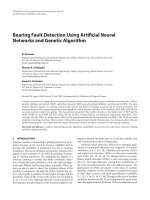
</div>Trang 13<div class="page_container" data-page="13">

Figure 1.1: Illustration of the adaptive graph convolutional layer (AGCL)

Where: Kv is set to 3; wk is the weight; G: is the gate controls res(1x1): residual connection. If the number of input channels is different from the number of the output channels, it will be inserted to transform the input to match the output in the channel dimension.

Attention module

The authors suggest an STC-attention module. It contains three sub-modules: spatial, temporal, and channel attention module.

</div>Trang 14<div class="page_container" data-page="14">

Figure 1.2: Illustration of the STC-attention module

Three sub-modules are arranged sequentially in SAM, TAM, and CAM orders. ⊗ denotes element-wise multiplication. ⊕ denotes the element-wise addition.

Spatial attention module (SAM)

The symbols are similar to the above Eq.

Channel attention module (CAM)

𝑀

𝑐

= 𝜎(𝑊

2

(𝛿 (𝑊

1

(𝐴𝑣𝑔𝑃𝑜𝑜𝑙(𝑓

𝑖𝑛

))))

Where: 𝑊1 and 𝑊2 are the weights of two fully-connected layers; 𝛿 (𝑑𝑒𝑙𝑡𝑎): is the ReLU activation function.

Basic block

</div>Trang 15<div class="page_container" data-page="15">

Figure 1.3: Illustration of the basic block.

Both the spatial GCN and the temporal GCN are followed by a batch normalization (BN) and a ReLU layer. A basic block is the series of one Spatial GCN (Convs), one STC attention module (STC), and one temporal GCN (Convt). A residual connection is added for each basic block to stabilize the training and gradient propagation.

Network architecture

The overall architecture of the network is the stack of these basic blocks. There

are a total of 9 blocks. The numbers of output channels for each block are 64, 64, 64,

128, 128, 128, 256, 256, 256. The BN layer batch normalization is added at the

beginning to normalize the input data. A global average pooling layer (GAP) is used The final output is sent to a softmax classifier to obtain the prediction.

</div>Trang 16<div class="page_container" data-page="16">

Figure 1.4: Illustration of the network architecture.

There are a total of 9 basic blocks (B1-B9). The three numbers of each block represent the number of input channels, the number of output channels, and the stride, respectively. GAP represents the global average pooling layer.

Multi-stream network

The first-order information (the coordinates of the joints), second-order information (the direction and length of the bones), and their motion information should

be investigated for the action recognition task.

In this paper, they model these four modalities in a multi-stream framework. In particular, they define that the joint closer to the center of gravity is the root joint, and the joint father is the target joint. Each bone is represented as a vector pointing from its root joint to its target joint. For example, the root joint in frame t is: vi,t =(xi,t, yi,t, zi,t) and the target joint is vj,t = (xj,t, yj,t, zj,t), so the vector of bone is calculated as ei,j,j = (xi,t− xj,t, yi,t − yj,t, zi,t− zj,t)

For the motion information, it is calculated as the difference between the same joints, or

</div>Trang 17<div class="page_container" data-page="17">

(xi,t, yi,t, zi,t), and in frame t+1, it is: vi,t+1 = (xi,t+1, yi,t+1, zi,t+1), so the motion information is: mi,t,t+1 = (xi,t+1− xi,t, yi,t+1− yi,t, zi,t+1− zi,t)

The overall architecture (MS-AAGCN) is shown in Fig:

Figure 1.5 Illustration of the overall architecture of the MS-AAGCN.

The four modalities (joints, bones, and their motions) are fed into four streams. Finally, the softmax scores of the four streams are used to obtain the action scores and predict the action label.

1.2.2. An Effective Pre-processing of High-order Skeletal Joint Feature Extraction to Enhance Graph-Convolution-Network-Based Action Recognition

In this work, Lie et al. considered the joints as vertices and the limbs/bones as edges, a human skeleton can be modeled as a graph, and they supposed pre-processing to boost the performance of GCN-based methods by enriching the skeletal joint information with high-order attributes.

They used GCN for action recognition but improve towards providing rich (RICH) or higher-order (up to order-3) joint information in the spatial and temporal domain, and feed them as the input to GCN networks in two ways:

1. Early fusion 2. Late fusion

• Early fusion and late fusion

</div>Trang 18<div class="page_container" data-page="18">

Figure 1.6: Multi-streams late fusion with RICH joint features.

Figure 1.7: Single streams early fusion with RICH joint features

About providing rich (RICH) or higher-order (up to order-3) joint information in the spatial and temporal domain:

• Order 1-3 joint spatial information

1. 𝟏𝒔𝒕 order(𝑺𝟏): Each joint j is described by a directed 3D vector-J from the

specified root joint (here, the spine) to its position.

</div>Trang 19<div class="page_container" data-page="19">

Figure 1.8: Definitions of vector-J of a joint.

2. 𝟐𝒏𝒅 order(𝑺𝟐): Each joint j is associated with a physical skeletal edge (human

bone) described by a directed 3D vector-E from a specified start joint (i.e., joint j is considered as the end of the vector). When selecting the start/end ordered joint pairs, they are made sure that the edge vector is pointing radially outwards away from the root.

Figure 1.9: Definitions of vector-E of a joint.

</div>