“Mechanics of Solids” Mechanical Engineering Handbook Ed. Frank pptx

Sandor, B.I.; Roloff, R; et. al. “Mechanics of Solids”
Mechanical Engineering Handbook
Ed. Frank Kreith
Boca Raton: CRC Press LLC, 1999
c

1999byCRCPressLLC

1

-1

© 1999 by CRC Press LLC

Mechanics of Solids

1.1 Introduction 1-1
1.2 Statics 1-3

Vectors. Equilibrium of Particles. Free-body Diagrams • Forces
on Rigid Bodies • Equilibrium of Rigid Bodies • Forces and
Moments in Beams • Simple Structures and Machines •
Distributed Forces • Friction • Work and Potential Energy •
Moments of Inertia

1.3 Dynamics 1-31

Kinematics of Particles • Kinetics of Particles • Kinetics of
Systems of Particles • Kinematics of Rigid Bodies • Kinetics
of Rigid Bodies in Plane Motion • Energy and Momentum
Methods for Rigid Bodies in Plane Motion • Kinetics of Rigid

Bodies in Three Dimensions

1.4 Vibrations 1-57

Undamped Free and Forced Vibrations • Damped Free and
Forced Vibrations • Vibration Control • Random Vibrations.
Shock Excitations • Multiple-Degree-of-Freedom Systems.
Modal Analysis • Vibration-Measuring Instruments

1.5 Mechanics of Materials 1-67

Stress • Strain • Mechanical Behaviors and Properties of
Materials • Uniaxial Elastic Deformations • Stresses in Beams
• Deflections of Beams • Torsion • Statically Indeterminate
Members • Buckling • Impact Loading • Combined Stresses •
Pressure Vessels • Experimental Stress Analysis and
Mechanical Testing

1.6 Structural Integrity and Durability 1-104

Finite Element Analysis. Stress Concentrations • Fracture
Mechanics • Creep and Stress Relaxation • Fatigue

1.7 Comprehensive Example of Using Mechanics of Solids
Methods 1-125

The Project • Concepts and Methods

1.1Introduction

Bela I. Sandor

Engineers use the concepts and methods of mechanics of solids in designing and evaluating tools,
machines, and structures, ranging from wrenches to cars to spacecraft. The required educational back-
ground for these includes courses in statics, dynamics, mechanics of materials, and related subjects. For
example, dynamics of rigid bodies is needed in generalizing the spectrum of service loads on a car,
which is essential in defining the vehicle’s deformations and long-term durability. In regard to structural

Bela I. Sandor

University of Wisconsin-Madison

Ryan Roloff

Allied Signal Aerospace

Stephen M. Birn

Allied Signal Aerospace

Maan H. Jawad

Nooter Consulting Services

Michael L. Brown

A.O. Smith Corp.

1

-2

Section 1

integrity and durability, the designer should think not only about preventing the catastrophic failures of
products, but also of customer satisfaction. For example, a car with gradually loosening bolts (which is
difficult to prevent in a corrosive and thermal and mechanical cyclic loading environment) is a poor
product because of safety, vibration, and noise problems. There are sophisticated methods to assure a
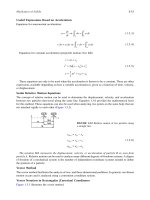
product’s performance and reliability, as exemplified in Figure 1.1.1. A similar but even more realistic
test setup is shown in Color Plate 1.

*

It is common experience among engineers that they have to review some old knowledge or learn
something new, but what is needed at the moment is not at their fingertips. This chapter may help the
reader in such a situation. Within the constraints of a single book on mechanical engineering, it provides
overviews of topics with modern perspectives, illustrations of typical applications, modeling to solve
problems quantitatively with realistic simplifications, equations and procedures, useful hints and remind-
ers of common errors, trends of relevant material and mechanical system behaviors, and references to
additional information.
The chapter is like an emergency toolbox. It includes a coherent assortment of basic tools, such as
vector expressions useful for calculating bending stresses caused by a three-dimensional force system
on a shaft, and sophisticated methods, such as life prediction of components using fracture mechanics
and modern measurement techniques. In many cases much more information should be considered than
is covered in this chapter.

*

Color Plates 1 to 16 follow page 1-131.

FIGURE 1.1.1

Artist’s concept of a moving stainless steel roadway to drive the suspension system through a
spinning, articulated wheel, simulating three-dimensional motions and forces. (MTS Systems Corp., Minneapolis,
MN. With permission.) Notes: Flat-Trac

®

Roadway Simulator, R&D100 Award-winning system in 1993. See also
Color Plate 1.

*

Mechanics of Solids

1

-3

1.2Statics

Bela I. Sandor

Vectors. Equilibrium of Particles. Free-Body Diagrams

Two kinds of quantities are used in engineering mechanics. A scalar quantity has only magnitude (mass,
time, temperature, …). A vector quantity has magnitude and direction (force, velocity, ). Vectors are
represented here by arrows and bold-face symbols, and are used in analysis according to universally
applicable rules that facilitate calculations in a variety of problems. The vector methods are indispensable
in three-dimensional mechanics analyses, but in simple cases equivalent scalar calculations are sufficient.

Vector Components and Resultants. Parallelogram Law

A given vector

F

may be replaced by two or three other vectors that have the same net effect and
representation. This is illustrated for the chosen directions

m

and

n

for the components of

F

in two
dimensions (Figure 1.2.1). Conversely, two concurrent vectors

F

and

P

of the same units may be

combined to get a resultant

R

(Figure 1.2.2).
Any set of components of a vector

F

must satisfy the

parallelogram law

. According to Figure 1.2.1,
the law of sines and law of cosines may be useful.
(1.2.1)
Any number of concurrent vectors may be summed, mathematically or graphically, and in any order,
using the above concepts as illustrated in Figure 1.2.3.

FIGURE 1.2.1

Addition of concurrent vectors

F

and

P

.

FIGURE 1.2.2

Addition of concurrent, coplanar
vectors

A

,

B

, and

C

.

FIGURE 1.2.3

Addition of concurrent, coplanar vectors

A

,

B

, and

C

.
FF
F
FF
nm
nm
sin sin
sin
cos
αβ
αβ
αβ
==
°− +
()
[]
=+− °−+
()
[]
180
2 180
222
FFF
nm

1

-4

Section 1

Unit Vectors

Mathematical manipulations of vectors are greatly facilitated by the use of unit vectors. A unit vector

n

has a magnitude of unity and a defined direction. The most useful of these are the unit coordinate
vectors

i

,

j

, and

k

as shown in Figure 1.2.4.
The three-dimensional components and associated quantities of a vector

F

are shown in Figure 1.2.5.
The unit vector

n

is collinear with

F

.
The vector

F

is written in terms of its scalar components and the unit coordinate vectors,
(1.2.2)
where
The unit vector notation is convenient for the summation of concurrent vectors in terms of scalar or
vector components:
Scalar components of the resultant

R

:
(1.2.3)

FIGURE 1.2.4

Unit vectors in Cartesian coordinates (the same

i

,

j

,
and

k

set applies in a parallel

x

′

y

′

z

′

system of axes).

FIGURE 1.2.5

Three-dimensional components of a vector

F

.
Fijkn=++=FFF
xyz
F
FFF
xxyyzz
===
=++
FFF
FFFF
xyz
cos cos cosθθθ
222
n
nnn
xyz
xxyyzz
nn===
++=
cos cos cosθθθ
222
1
n
n
n
x
x
y
y
z

z
FFFF
===
1
RFRFRF
xxyyzz
===
∑∑∑

Mechanics of Solids

1

-5

Vector components:
(1.2.4)

Vector Determination from Scalar Information

A force, for example, may be given in terms of its magnitude

F

, its sense of direction, and its line of
action. Such a force can be expressed in vector form using the coordinates of any two points on its line
of action. The vector sought is
The method is to find

n

on the line of points

A

(

x

1

,

y

1

,

z

1

) and

B

(

x

2

,

y

2

,

z

2

):
where

d

x

=

x

2

–

x

1

,

d

y

=

y

2

–

y

1

,

d

z

=

z

2

–

z

1

.

Scalar Product of Two Vectors. Angles and Projections of Vectors

The scalar product, or dot product, of two concurrent vectors

A

and

B

is defined by
(1.2.5)
where

A

and

B

are the magnitudes of the vectors and

φ

is the angle between them. Some useful expressions
are
The projection

F

′

of a vector

F

on an arbitrary line of interest is determined by placing a unit vector

n on that line of interest, so that
Equilibrium of a Particle
A particle is in equilibrium when the resultant of all forces acting on it is zero. In such cases the
algebraic summation of rectangular scalar components of forces is valid and convenient:
(1.2.6)
Free-Body Diagrams
Unknown forces may be determined readily if a body is in equilibrium and can be modeled as a particle.
The method involves free-body diagrams, which are simple representations of the actual bodies. The
appropriate model is imagined to be isolated from all other bodies, with the significant effects of other
bodies shown as force vectors on the free-body diagram.

RFiRFjRFk
xxxyyyzzz
FFF== == ==
∑∑ ∑∑ ∑∑
Fijkn=++=FFF
xyz
F
n
ijk
==
++
++
vector A to B
distance A to B
d
ddd
xyz
xyz
dd
222
AB⋅=ABcosφ
ABBA⋅=⋅= + +
=
++
AB AB AB
AB AB AB
AB
xx yy zz
xx yy zz
φ arccos

′
=⋅= + +FFnFnFnFn
xx yy zz
FFF
xyz
∑∑∑
===000
1-6 Section 1
Example 1
A mast has three guy wires. The initial tension in each wire is planned to be 200 lb. Determine whether
this is feasible to hold the mast vertical (Figure 1.2.6).
Solution.
The three tensions of known magnitude (200 lb) must be written as vectors.
The resultant of the three tensions is
There is a horizontal resultant of 31.9 lb at A, so the mast would not remain vertical.
Forces on Rigid Bodies
All solid materials deform when forces are applied to them, but often it is reasonable to model components
and structures as rigid bodies, at least in the early part of the analysis. The forces on a rigid body are
generally not concurrent at the center of mass of the body, which cannot be modeled as a particle if the
force system tends to cause a rotation of the body.
FIGURE 1.2.6A mast with guy wires.
RTTT=++
AB AC AD
Tn
ijk
ijk i j k
AB AB
AB A B
d
d

=
()( )
==
++
()
=
++
−−+
()
=− − +
tension unit vector to lb lb
lb ft
ft
lb lb lb
200 200
200
5104
5 10 4 842 1684 674
222
xyz
dd

Tijkijk
AC
=−+
()
=++
200
1187
5 10 4 842 1684 674

lb
ft
ft lb lb lb
.

Tijkjk
AD
=−+
()
=− −
200
1166
0 10 6 1715 1029
lb
ft
ft lb lb
.

Rijk i j
kij k
=++=−++
()
+− − −
()
++−
()
=−+
∑∑∑
FFF
xyz

842842 0 168416841715
6746741029 0 508 319

.
lb lb
lb lb lb lb
Mechanics of Solids 1-7
Moment of a Force
The turning effect of a force on a body is called the moment of the force, or torque. The moment M
A
of a force F about a point A is defined as a scalar quantity
(1.2.7)
where d (the moment arm or lever arm) is the nearest distance from A to the line of action of F. This
nearest distance may be difficult to determine in a three-dimensional scalar analysis; a vector method
is needed in that case.
Equivalent Forces
Sometimes the equivalence of two forces must be established for simplifying the solution of a problem.
The necessary and sufficient conditions for the equivalence of forces F and F
′

are that they have the
same magnitude, direction, line of action, and moment on a given rigid body in static equilibrium. Thus,
For example, the ball joint A in Figure 1.2.7 experiences the same moment whether the vertical force
is pushing or pulling downward on the yoke pin.
Vector Product of Two Vectors
A powerful method of vector mechanics is available for solving complex problems, such as the moment
of a force in three dimensions. The vector product (or cross product) of two concurrent vectors A and
B is defined as the vector V = A × B with the following properties:
1.V is perpendicular to the plane of vectors A and B.
2.The sense of V is given by the right-hand rule (Figure 1.2.8).

3.The magnitude of V is V = AB sinθ, where θ is the angle between A and B.
4.A × B ≠ B × A, but A × B = –(B × A).
5.For three vectors, A × (B + C) = A × B + A × C.
FIGURE 1.2.7Schematic of testing a ball joint of a car.
FIGURE 1.2.8Right-hand rule for vector products.
MFd
A
=
FF=
′
=
′
and MM
AA
1-8 Section 1
The vector product is calculated using a determinant,
(1.2.8)
Moment of a Force about a Point
The vector product is very useful in determining the moment of a force F about an arbitrary point O.
The vector definition of moment is
(1.2.9)
where r is the position vector from point O to any point on the line of action of F. A double arrow is
often used to denote a moment vector in graphics.
The moment M
O
may have three scalar components, M
x
, M
y
, M

z
, which represent the turning effect
of the force F about the corresponding coordinate axes. In other words, a single force has only one
moment about a given point, but this moment may have up to three components with respect to a
coordinate system,
Triple Products of Three Vectors
Two kinds of products of three vectors are used in engineering mechanics. The mixed triple product (or
scalar product) is used in calculating moments. It is the dot product of vector A with the vector product
of vectors B and C,
(1.2.10)
The vector triple product (A × B) × C = V × C is easily calculated (for use in dynamics), but note that
Moment of a Force about a Line
It is common that a body rotates about an axis. In that case the moment M
ᐉ
of a force F about the axis,
say line ᐉ, is usefully expressed as
(1.2.11)
where n is a unit vector along the line ᐉ, and r is a position vector from point O on ᐉ to a point on the
line of action of F. Note that M
ᐉ
is the projection of M
O
on line ᐉ.
V
ijk
ijkkji==++−−−AAA
BBB
AB AB AB AB AB AB
xyz
xyz

yz zx xy yx xz zy
MrF
O
=×
Mijk
Ox y z
MMM=++
ABC⋅×
()
==−
()
+−
()
+−
()
AAA
BBB
CCC
ABC BC ABC BC ABC BC
xyz
xyz
xyz
xyz zy yzx xz zxy yx
AB CA BC×
()
×≠× ×
()

MnM nrF
l

=⋅ =⋅ ×
()
=
O
xyz
xyz
xyz
nnn
rrr
FFF
Mechanics of Solids 1-9
Special Cases
1.The moment about a line ᐉ is zero when the line of action of F intersects ᐉ (the moment arm is
zero).
2.The moment about a line ᐉ is zero when the line of action of F is parallel to ᐉ (the projection of
M
O
on ᐉ is zero).
Moment of a Couple
A pair of forces equal in magnitude, parallel in lines of action, and opposite in direction is called a
couple. The magnitude of the moment of a couple is
where d is the distance between the lines of action of the forces of magnitude F. The moment of a couple
is a free vector M that can be applied anywhere to a rigid body with the same turning effect, as long
as the direction and magnitude of M are the same. In other words, a couple vector can be moved to any
other location on a given rigid body if it remains parallel to its original position (equivalent couples).
Sometimes a curled arrow in the plane of the two forces is used to denote a couple, instead of the couple
vector M, which is perpendicular to the plane of the two forces.
Force-Couple Transformations
Sometimes it is advantageous to transform a force to a force system acting at another point, or vice
versa. The method is illustrated in Figure 1.2.9.

1.A force F acting at B on a rigid body can be replaced by the same force F acting at A and a
moment M
A
= r

× F about A.
2.A force F and moment M
A
acting at A can be replaced by a force F acting at B for the same total
effect on the rigid body.
Simplification of Force Systems
Any force system on a rigid body can be reduced to an equivalent system of a resultant force R and a
resultant moment M
R
. The equivalent force-couple system is formally stated as
(1.2.12)
where M
R
depends on the chosen reference point.
Common Cases
1.The resultant force is zero, but there is a resultant moment: R = 0, M
R
≠ 0.
2.Concurrent forces (all forces act at one point): R ≠ 0, M
R
= 0.
3.Coplanar forces: R ≠ 0, M
R
≠ 0. M
R

is perpendicular to the plane of the forces.
4.Parallel forces: R ≠ 0, M
R
≠ 0. M
R
is perpendicular to R.
FIGURE 1.2.9Force-couple transformations.
MFd=
RFMMrF===×
()
===
∑∑∑
i
i
n
Ri
i
n
ii
i
n
111
and
1-10 Section 1
Example 2
The torque wrench in Figure 1.2.10 has an arm of constant length L but a variable socket length d =
OA because of interchangeable tool sizes. Determine how the moment applied at point O depends on
the length d for a constant force F from the hand.
Solution. Using M
O

= r × F with r = Li + dj and F = Fk in Figure 1.2.10,
Judgment of the Result
According to a visual analysis the wrench should turn clockwise, so the –j component of the moment
is justified. Looking at the wrench from the positive x direction, point A has a tendency to rotate
counterclockwise. Thus, the i component is correct using the right-hand rule.
Equilibrium of Rigid Bodies
The concept of equilibrium is used for determining unknown forces and moments of forces that act on
or within a rigid body or system of rigid bodies. The equations of equilibrium are the most useful
equations in the area of statics, and they are also important in dynamics and mechanics of materials.
The drawing of appropriate free-body diagrams is essential for the application of these equations.
Conditions of Equilibrium
A rigid body is in static equilibrium when the equivalent force-couple system of the external forces
acting on it is zero. In vector notation, this condition is expressed as
(1.2.13)
where O is an arbitrary point of reference.
In practice it is often most convenient to write Equation 1.2.13 in terms of rectangular scalar com-
ponents,
FIGURE 1.2.10Model of a torque wrench.
Mijkij
O
LdFFdFL=+
()
×=−
F
MrF
∑
∑∑
=
=×
()

=
0
0
O
FM
FM
FM
xx
yy
zz
∑∑
∑∑
∑∑
==
==
==
00
00
00
Mechanics of Solids 1-11
Maximum Number of Independent Equations for One Body
1.One-dimensional problem: ∑F = 0
2.Two-dimensional problem:
3.Three-dimensional problem:
where xyz are orthogonal coordinate axes, and A, B, C are particular points of reference.
Calculation of Unknown Forces and Moments
In solving for unknown forces and moments, always draw the free-body diagram first. Unknown external
forces and moments must be shown at the appropriate places of action on the diagram. The directions
of unknowns may be assumed arbitrarily, but should be done consistently for systems of rigid bodies.
A negative answer indicates that the initial assumption of the direction was opposite to the actual

direction. Modeling for problem solving is illustrated in Figures 1.2.11 and 1.2.12.
Notes on Three-Dimensional Forces and Supports
Each case should be analyzed carefully. Sometimes a particular force or moment is possible in a device,
but it must be neglected for most practical purposes. For example, a very short sleeve bearing cannot
FIGURE 1.2.11Example of two-dimensional modeling.
FIGURE 1.2.12Example of three-dimensional modeling.

FFM
FMMx
MMMAB
xyA
xAB
ABC
∑∑∑
∑∑∑
∑∑∑
===
===
===
000
000
000
or axis not AB)
or not BC)
(
(
⊥
࿣
FFF
MMM

xyz
xyz
∑∑∑
∑∑∑
===
===
000
000
1-12 Section 1
support significant moments. A roller bearing may be designed to carry much larger loads perpendicular
to the shaft than along the shaft.
Related Free-Body Diagrams
When two or more bodies are in contact, separate free-body diagrams may be drawn for each body. The
mutual forces and moments between the bodies are related according to Newton’s third law (action and
reaction). The directions of unknown forces and moments may be arbitrarily assumed in one diagram,
but these initial choices affect the directions of unknowns in all other related diagrams. The number of
unknowns and of usable equilibrium equations both increase with the number of related free-body
diagrams.
Schematic Example in Two Dimensions (Figure 1.2.13)
Given: F
1
, F
2
, F
3
, M
Unknowns: P
1
, P
2

, P
3
, and forces and moments at joint A (rigid connection)
Equilibrium Equations
Three unknowns (P
1
, P
2
, P
3
) are in three equations.
Related Free-Body Diagrams (Figure 1.2.14)
Dimensions a, b, c, d, and e of Figure 1.2.13 are also valid here.
FIGURE 1.2.13Free-body diagram.
FIGURE 1.2.14Related free-body diagrams.
FFP
FPPFF
MPcPcdeMFaFab
x
y
O
∑
∑
∑
=−+ =
=+−−=
=+++
()
+−−+
()

=
13
1223
12 23
0
0
0
Mechanics of Solids 1-13
New Set of Equilibrium Equations
Six unknowns (P
1
, P
2
, P
3
, A
x
, A
y
, M
A
) are in six equations.
Note: In the first diagram (Figure 1.2.13) the couple M may be moved anywhere from O to B. M is
not shown in the second diagram (O to A) because it is shown in the third diagram (in which it may be
moved anywhere from A to B).
Example 3
The arm of a factory robot is modeled as three bars (Figure 1.2.15) with coordinates A: (0.6, –0.3, 0.4)
m; B: (1, –0.2, 0) m; and C: (0.9, 0.1, –0.25) m. The weight of the arm is represented by W
A
= –60 Nj

at A, and W
B
= –40 Nj at B. A moment M
C
= (100i – 20j + 50k) N · m is applied to the arm at C.
Determine the force and moment reactions at O, assuming that all joints are temporarily fixed.
Solution. The free-body diagram is drawn in Figure 1.2.15b, showing the unknown force and moment
reactions at O. From Equation 1.2.13,
FIGURE 1.2.15Model of a factory robot.
Left part:
Right side:
OA
FFA
FPAF
MPcAcdMFa
AB
FAP
FPAF
MMPeMFf
xx
yy
Oy A
xx
yy
AA
()
=−+ =
=+−=
=++
()

+−=
()
=− + =
=−−=
=− + + − =
∑
∑
∑
∑
∑
∑
1
12
12
3
23
23
0
0
0
0
0
0
F
∑
=0
FWW
OAB
++=0
Fjj

O
−−=60 40 0 N N
1-14 Section 1
Example 4
A load of 7 kN may be placed anywhere within A and B in the trailer of negligible weight. Determine
the reactions at the wheels at D, E, and F, and the force on the hitch H that is mounted on the car, for
the extreme positions A and B of the load. The mass of the car is 1500 kg, and its weight is acting at
C (see Figure 1.2.16).
Solution. The scalar method is best here.
Forces and Moments in Beams
Beams are common structural members whose main function is to resist bending. The geometric changes
and safety aspects of beams are analyzed by first assuming that they are rigid. The preceding sections
enable one to determine (1) the external (supporting) reactions acting on a statically determinate beam,
and (2) the internal forces and moments at any cross section in a beam.
FIGURE 1.2.16Analysis of a car with trailer.
Put the load at position A first
For the trailer alone, with y as the vertical axis
∑M
F
= 7(1) – H
y
(3) = 0, H
y
= 2.33 kN
On the car
H
y
= 2.33 kN ↓Ans.
∑F
y

= 2.33 – 7 + F
y
= 0, F
y
= 4.67 kN ↑Ans.
For the car alone
∑M
E
= –2.33(1.2) – D
y
(4) + 14.72(1.8) = 0
D
y
= 5.93 kN ↑Ans.
∑F
y
= 5.93 + E
y
– 14.72 – 2.33 = 0
E
y
= 11.12 kN ↑Ans.
Put the load at position B next
For the trailer alone
∑M
F
= 0.8(7) – H
y
(3) = 0, H
y

= –1.87 kN
On the car
H
y
= 1.87 kN ↓Ans.
∑F
y
= –1.87 – 7 + E
y
= 0
E
y
= 8.87 kN ↑Ans.
For the car alone
∑M
E
= –(1.87)(1.2) – D
y
(4) + 14.72(1.8) = 0
D
y
= 7.19 kN ↑Ans.
∑F
y
= 7.19 + E
y
– 14.72 – (–1.87) = 0
E
y
= 5.66 kN ↑Ans.

Fj
O
=100 N
M
O
∑
=0
MMrWrW
OCOAAOBB
++×
()
+×
()
=0
Mijk ijk jij j
O
+−+
()
⋅+ −+
()
×−
()
+−
()
×−
()
=100 20 50 06 03 04 60 02 40 0 Nm m N m N .
Mijkkik
O
+⋅−⋅+⋅−⋅+⋅−⋅=100 20 50 36 24 40 0 Nm Nm Nm Nm Nm Nm

Mijk
O
=− + +
()
⋅124 20 26 Nm
Mechanics of Solids 1-15
Classification of Supports
Common supports and external reactions for two-dimensional loading of beams are shown in Figure
1.2.17.
Internal Forces and Moments
The internal force and moment reactions in a beam caused by external loading must be determined for
evaluating the strength of the beam. If there is no torsion of the beam, three kinds of internal reactions
are possible: a horizontal normal force H on a cross section, vertical (transverse) shear force V, and
bending moment M. These reactions are calculated from the equilibrium equations applied to the left
or right part of the beam from the cross section considered. The process involves free-body diagrams
of the beam and a consistently applied system of signs. The modeling is illustrated for a cantilever beam
in Figure 1.2.18.
Sign Conventions. Consistent sign conventions should be used in any given problem. These could be
arbitrarily set up, but the following is slightly advantageous. It makes the signs of the answers to the
equilibrium equations correct for the directions of the shear force and bending moment.
A moment that makes a beam concave upward is taken as positive. Thus, a clockwise moment is
positive on the left side of a section, and a counterclockwise moment is positive on the right side. A
FIGURE 1.2.17Common beam supports.
FIGURE 1.2.18Internal forces and moments in a cantilever beam.
1-16 Section 1
shear force that acts upward on the left side of a section, or downward on the right side, is positive
(Figure 1.2.19).
Shear Force and Bending Moment Diagrams
The critical locations in a beam are determined from shear force and bending moment diagrams for the
whole length of the beam. The construction of these diagrams is facilitated by following the steps

illustrated for a cantilever beam in Figure 1.2.20.
1.Draw the free-body diagram of the whole beam and determine all reactions at the supports.
2.Draw the coordinate axes for the shear force (V) and bending moment (M) diagrams directly
below the free-body diagram.
3.Immediately plot those values of V and M that can be determined by inspection (especially where
they are zero), observing the sign conventions.
4.Calculate and plot as many additional values of V and M as are necessary for drawing reasonably
accurate curves through the plotted points, or do it all by computer.
Example 5
A construction crane is modeled as a rigid bar AC which supports the boom by a pin at B and wire CD.
The dimensions are AB = 10ᐉ, BC = 2ᐉ, BD = DE = 4ᐉ. Draw the shear force and bending moment
diagrams for bar AC (Figure 1.2.21).
Solution. From the free-body diagram of the entire crane,
FIGURE 1.2.19Preferred sign conventions.
FIGURE 1.2.20Construction of shear force and bending moment diagrams.

FF M
APAPM
AP MP
xy A
xy A
yA
∑∑ ∑
== =
=−+=−
()
+=
==
00 0
0080

8
l
l
Mechanics of Solids 1-17
Now separate bar AC and determine the forces at B and C.
From (a) and (c), B
x
= 4P and = 4P. From (b) and (c), B
y
= P – 2P = –P and = 2P.
Draw the free-body diagram of bar AC horizontally, with the shear force and bending moment diagram
axes below it. Measure x from end C for convenience and analyze sections 0 ≤ x ≤ 2ᐉ and 2ᐉ ≤ x ≤ 12ᐉ
(Figures 1.2.21b to 1.2.21f).
1.0 ≤ x ≤ 2ᐉ
2.2ᐉ ≤ x ≤ 12ᐉ
FIGURE 1.2.21Shear force and bending moment diagrams of a component in a structure.

FF M
BT PBT T B M
BT BPT TTP
TPP
xy A
x CD y CD CD x A
x CD y CD CD CD
CD
xy
∑∑ ∑
== =
−+= −−= −
()

+
()
+=
==−−+=−
==
00 0
00
2
5
12 10 0
2
5
1
5
24
5
20
5
8
85
4
25
ll
ll
l() ()
()
ab
c
T
CD

x
T
CD
y
FM
PV M Px
VP MPx
yK
KK
KK
∑∑
==
−+= +
()
=
==−
00
40 40
44
11
11
1-18 Section 1
At point B, x = 2ᐉ,= –4P(2ᐉ) = –8Pᐉ == M
A
. The results for section AB, 2ᐉ ≤ x ≤ 12ᐉ, show
that the combined effect of the forces at B and C is to produce a couple of magnitude 8Pᐉ on the beam.
Hence, the shear force is zero and the moment is constant in this section. These results are plotted on
the axes below the free-body diagram of bar A-B-C.
Simple Structures and Machines
Ryan Roloff and Bela I. Sandor

Equilibrium equations are used to determine forces and moments acting on statically determinate simple
structures and machines. A simple structure is composed solely of two-force members. A machine is
composed of multiforce members. The method of joints and the method of sections are commonly used
in such analysis.
Trusses
Trusses consist of straight, slender members whose ends are connected at joints. Two-dimensional plane
trusses carry loads acting in their planes and are often connected to form three-dimensional space trusses.
Two typical trusses are shown in Figure 1.2.22.
To simplify the analysis of trusses, assume frictionless pin connections at the joints. Thus, all members
are two-force members with forces (and no moments) acting at the joints. Members may be assumed
weightless or may have their weights evenly divided to the joints.
Method of Joints
Equilibrium equations based on the entire truss and its joints allow for determination of all internal
forces and external reactions at the joints using the following procedure.
1.Determine the support reactions of the truss. This is done using force and moment equilibrium
equations and a free-body diagram of the entire truss.
2.Select any arbitrary joint where only one or two unknown forces act. Draw the free-body diagram
of the joint assuming unknown forces are tensions (arrows directed away from the joint).
3.Draw free-body diagrams for the other joints to be analyzed, using Newton’s third law consistently
with respect to the first diagram.
4.Write the equations of equilibrium, ∑F
x
= 0 and ∑F
y
= 0, for the forces acting at the joints and
solve them. To simplify calculations, attempt to progress from joint to joint in such a way that
each equation contains only one unknown. Positive answers indicate that the assumed directions
of unknown forces were correct, and vice versa.
Example 6
Use the method of joints to determine the forces acting at A, B, C, H, and I of the truss in Figure 1.2.23a.

The angles are α = 56.3°, β = 38.7°, φ = 39.8°, and θ = 36.9°.
FIGURE 1.2.22Schematic examples of trusses.

FM
P PV M Px Px
VMP
yK
KK
KK
∑∑
==
−+= −−
()
+
()
=
==−
00
44 0 424 0
08
22
22
l
l
M
K
1
M
K
2

Mechanics of Solids 1-19
Solution. First the reactions at the supports are determined and are shown in Figure 1.2.23b. A joint at
which only two unknown forces act is the best starting point for the solution. Choosing joint A, the
solution is progressively developed, always seeking the next joint with only two unknowns. In each
diagram circles indicate the quantities that are known from the preceding analysis. Sample calculations
show the approach and some of the results.
Method of Sections
The method of sections is useful when only a few forces in truss members need to be determined
regardless of the size and complexity of the entire truss structure. This method employs any section of
the truss as a free body in equilibrium. The chosen section may have any number of joints and members
in it, but the number of unknown forces should not exceed three in most cases. Only three equations of
equilibrium can be written for each section of a plane truss. The following procedure is recommended.
1.Determine the support reactions if the section used in the analysis includes the joints supported.
FIGURE 1.2.23Method of joints in analyzing a truss.
Joint A:
kips
kips (tension)
FF
FFA
F
F
xy
AI AB y
AB
AB
∑∑
==
=−=
−=
=

00
00
50 0
50
Joint H: FF
xy
∑∑
==00
FFF FFFF
FF
FF
GH CH BH CH DH GH HI
GH DH
GH DH
sin cos sin cos


βα α β−−= ++−=
()
+
()
()
−=−
()
()
+−
()
()
+
=− =

00
0625 601 0555 0 0 601 0832 534 0780 70
534 217
kips kips kips kips=0
kips (compression) kips (tension)
1-20 Section 1
2.Section the truss by making an imaginary cut through the members of interest, preferably through
only three members in which the forces are unknowns (assume tensions). The cut need not be a
straight line. The sectioning is illustrated by lines l-l, m-m, and n-n in Figure 1.2.24.
3.Write equations of equilibrium. Choose a convenient point of reference for moments to simplify
calculations such as the point of intersection of the lines of action for two or more of the unknown
forces. If two unknown forces are parallel, sum the forces perpendicular to their lines of action.
4.Solve the equations. If necessary, use more than one cut in the vicinity of interest to allow writing
more equilibrium equations. Positive answers indicate assumed directions of unknown forces were
correct, and vice versa.
Space Trusses
A space truss can be analyzed with the method of joints or with the method of sections. For each joint,
there are three scalar equilibrium equations, ∑F
x
= 0, ∑F
y
= 0, and ∑F
z
= 0. The analysis must begin
at a joint where there are at least one known force and no more than three unknown forces. The solution
must progress to other joints in a similar fashion.
There are six scalar equilibrium equations available when the method of sections is used: ∑F
x
= 0,
∑F

y
= 0, ∑F
z
= 0, ∑M
x
= 0, ∑M
y
= 0, and ∑M
z
= 0.
Frames and Machines
Multiforce members (with three or more forces acting on each member) are common in structures. In
these cases the forces are not directed along the members, so they are a little more complex to analyze
than the two-force members in simple trusses. Multiforce members are used in two kinds of structure.
Frames are usually stationary and fully constrained. Machines have moving parts, so the forces acting
on a member depend on the location and orientation of the member.
The analysis of multiforce members is based on the consistent use of related free-body diagrams. The
solution is often facilitated by representing forces by their rectangular components. Scalar equilibrium
equations are the most convenient for two-dimensional problems, and vector notation is advantageous
in three-dimensional situations.
Often, an applied force acts at a pin joining two or more members, or a support or connection may
exist at a joint between two or more members. In these cases, a choice should be made of a single
member at the joint on which to assume the external force to be acting. This decision should be stated
in the analysis. The following comprehensive procedure is recommended.
Three independent equations of equilibrium are available for each member or combination of members
in two-dimensional loading; for example, ∑F
x
= 0, ∑F
y
= 0, ∑M

A
= 0, where A is an arbitrary point of
reference.
1.Determine the support reactions if necessary.
2.Determine all two-force members.
FIGURE 1.2.24Method of sections in analyzing a truss.
Mechanics of Solids 1-21
3. Draw the free-body diagram of the first member on which the unknown forces act assuming that
the unknown forces are tensions.
4. Draw the free-body diagrams of the other members or groups of members using Newton’s third
law (action and reaction) consistently with respect to the first diagram. Proceed until the number
of equilibrium equations available is no longer exceeded by the total number of unknowns.
5. Write the equilibrium equations for the members or combinations of members and solve them.
Positive answers indicate that the assumed directions for unknown forces were correct, and vice
versa.
Distributed Forces
The most common distributed forces acting on a body are parallel force systems, such as the force of
gravity. These can be represented by one or more concentrated forces to facilitate the required analysis.
Several basic cases of distributed forces are presented here. The important topic of stress analysis is
covered in mechanics of materials.
Center of Gravity
The center of gravity of a body is the point where the equivalent resultant force caused by gravity is
acting. Its coordinates are defined for an arbitrary set of axes as
(1.2.14)
where x, y, z are the coordinates of an element of weight dW, and W is the total weight of the body. In
the general case dW = γ dV, and W = ∫γ dV, where γ = specific weight of the material and dV = elemental
volume.
Centroids
If γ is a constant, the center of gravity coincides with the centroid, which is a geometrical property of
a body. Centroids of lines L, areas A, and volumes V are defined analogously to the coordinates of the

center of gravity,
For example, an area A consists of discrete parts A
1
, A
2
, A
3
, where the centroids x
1
, x
2
, x
3
of the three
parts are located by inspection. The x coordinate of the centroid of the whole area A is obtained from
= A
1
x
1
+ A
2
x
2
+ A
3
x
3
.
x
xdW

W
y
ydW
W
z
zdW
W
===
∫∫∫
Lines: = = =x
xdL
W
y
ydL
L
z
zdL
L
∫∫∫
( )1215
Areas: = = =x
xdA
A
y
ydA
A
z
zdA
A
∫∫∫

( )1216
Volumes: = = =x
xdV
V
y
ydV
V
z
zdV
V
∫∫∫
( )1217
x
Ax
1-22 Section 1
Surfaces of Revolution. The surface areas and volumes of bodies of revolution can be calculated using
the concepts of centroids by the theorems of Pappus (see texts on Statics).
Distributed Loads on Beams
The distributed load on a member may be its own weight and/or some other loading such as from ice
or wind. The external and internal reactions to the loading may be determined using the condition of
equilibrium.
External Reactions. Replace the whole distributed load with a concentrated force equal in magnitude to
the area under the load distribution curve and applied at the centroid of that area parallel to the original
force system.
Internal Reactions. For a beam under a distributed load w(x), where x is distance along the beam, the
shear force V and bending moment M are related according to Figure 1.2.25 as
(1.2.18)
Other useful expressions for any two cross sections A and B of a beam are
(1.2.19)
Example 7 (Figure 1.2.26)

Distributed Loads on Flexible Cables
The basic assumptions of simple analyses of cables are that there is no resistance to bending and that
the internal force at any point is tangent to the cable at that point. The loading is denoted by w(x), a
FIGURE 1.2.25Internal reactions in a beam under distributed loading.
FIGURE 1.2.26Shear force and bending moment diagrams for a cantilever beam.
wx
dV
dx
V
dM
dx
()
=− =
V V wxdx wx
MM Vdx
AB
x
x
BA
x
x
A
B
A
B
−=
()
=
()
−= =

∫
∫
area under
area under shear force diagram
Mechanics of Solids 1-23
continuous but possibly variable load, in terms of force per unit length. The differential equation of a
cable is
(1.2.20)
where T
o
= constant = horizontal component of the tension T in the cable.
Two special cases are common.
Parabolic Cables. The cable supports a load w which is uniformly distributed horizontally. The shape
of the cable is a parabola given by
(1.2.21)
In a symmetric cable the tension is .
Catenary Cables. When the load w is uniformly distributed along the cable, the cable’s shape is given by
(1.2.22)
The tension in the cable is T = T
o
+ wy.
Friction
A friction force F (or Ᏺ, in typical other notation) acts between contacting bodies when they slide
relative to one another, or when sliding tends to occur. This force is tangential to each body at the point
of contact, and its magnitude depends on the normal force N pressing the bodies together and on the
material and condition of the contacting surfaces. The material and surface properties are lumped together
and represented by the coefficient of friction µ. The friction force opposes the force that tends to cause
motion, as illustrated for two simple cases in Figure 1.2.27.
The friction forces F may vary from zero to a maximum value,
(1.2.23)

depending on the applied force that tends to cause relative motion of the bodies. The coefficient of
kinetic friction µ
k
(during sliding) is lower than the coefficient of static friction µ or µ
s
; µ
k
depends on
the speed of sliding and is not easily quantified.
FIGURE 1.2.27Models showing friction forces.
dy
dx
wx
T
o
2
2
=
()
y
wx
T
x
o
==
()
2
2
0 at lowest point
TTwx

o
=+
222
y
T
w
wx
T
o
o
=−






cosh 1
FNFF
max max
=≤≤
()
µ 0
1-24 Section 1
Angle of Repose
The critical angle θ
c
at which motion is impending is the angle of repose, where the friction force is at
its maximum for a given block on an incline.
(1.2.24)

So θ
c
is measured to obtain µ
s
. Note that, even in the case of static, dry friction, µ
s
depends on temperature,
humidity, dust and other contaminants, oxide films, surface finish, and chemical reactions. The contact
area and the normal force affect µ
s
only when significant deformations of one or both bodies occur.
Classifications and Procedures for Solving Friction Problems
The directions of unknown friction forces are often, but not always, determined by inspection. The
magnitude of the friction force is obtained from F
max
= µ
s
N when it is known that motion is impending.
Note that F may be less than F
max
. The major steps in solving problems of dry friction are organized in
three categories as follows.
Wedges and Screws
A wedge may be used to raise or lower a body. Thus, two directions of motion must be considered in
each situation, with the friction forces always opposing the impending or actual motion. The self-locking
A. Given: Bodies, forces, or coefficients of friction are known. Impending motion is
not assured: F ≠ µ
s
N.
Procedure: To determine if equilibrium is possible:

1. Construct the free-body diagram.
2. Assume that the system is in equilibrium.
3. Determine the friction and normal forces necessary for equilibrium.
4. Results: (a) F < µ
s
N, the body is at rest.
(b) F > µ
s
N, motion is occurring, static equilibrium is not
possible. Since there is motion, F = µ
k
N. Complete
solution requires principles of dynamics.
B. Given: Bodies, forces, or coefficients of friction are given. Impending motion is
specified. F = µ
s
N is valid.
Procedure: To determine the unknowns:
1. Construct the free-body diagram.
2. Write F = µ
s
N for all surfaces where motion is impending.
3. Determine µ
s
or the required forces from the equation of equilibrium.
C. Given: Bodies, forces, coefficients of friction are known. Impending motion is
specified, but the exact motion is not given. The possible motions may be
sliding, tipping or rolling, or relative motion if two or more bodies are
involved. Alternatively, the forces or coefficients of friction may have to be
determined to produce a particular motion from several possible motions.

Procedure: To determine the exact motion that may occur, or unknown quantities
required:
1. Construct the free-body diagram.
2. Assume that motion is impending in one of the two or more possible
ways. Repeat this for each possible motion and write the equation of
equilibrium.
3. Compare the results for the possible motions and select the likely event.
Determine the required unknowns for any preferred motion.
tanθµ
cs
F
N
==