Tài liệu Mechanical Engineering Handbook P2 docx
Bạn đang xem bản rút gọn của tài liệu. Xem và tải ngay bản đầy đủ của tài liệu tại đây (143.02 KB, 10 trang )
Mechanics of Solids 1-33
Useful Expressions Based on Acceleration
Equations for nonconstant acceleration:
(1.3.3)
(1.3.4)
Equations for constant acceleration (projectile motion; free fall):
(1.3.5)
These equations are only to be used when the acceleration is known to be a constant. There are other
expressions available depending on how a variable acceleration is given as a function of time, velocity,
or displacement.
Scalar Relative Motion Equations
The concept of relative motion can be used to determine the displacement, velocity, and acceleration
between two particles that travel along the same line. Equation 1.3.6 provides the mathematical basis
for this method. These equations can also be used when analyzing two points on the same body that are
not attached rigidly to each other (Figure 1.3.2).
(1.3.6)
The notation B/A represents the displacement, velocity, or acceleration of particle B as seen from
particle A. Relative motion can be used to analyze many different degrees-of-freedom systems. A degree
of freedom of a mechanical system is the number of independent coordinate systems needed to define
the position of a particle.
Vector Method
The vector method facilitates the analysis of two- and three-dimensional problems. In general, curvilinear
motion occurs and is analyzed using a convenient coordinate system.
Vector Notation in Rectangular (Cartesian) Coordinates
Figure 1.3.3 illustrates the vector method.
FIGURE 1.3.2Relative motion of two particles along
a straight line.
a
dv
dt
dv adt
v
vt
=⇒=
∫∫
0
0
vdvadx vdv adx
v
v
x
x
=⇒=
∫∫
00
vatv
vaxxv
xatvtx
=+
=−
()
+
=++
0
2
00
2
2
00
2
1
2
xxx
vvv
aaa
BA B A
BA B A
BA B A
=−
=−
=−
1-34 Section 1
The mathematical method is based on determining v and a as functions of the position vector r. Note
that the time derivatives of unit vectors are zero when the xyz coordinate system is fixed. The scalar
components can be determined from the appropriate scalar equations previously presented
that only include the quantities relevant to the coordinate direction considered.
(1.3.7)
There are a few key points to remember when considering curvilinear motion. First, the instantaneous
velocity vector is always tangent to the path of the particle. Second, the speed of the particle is the
magnitude of the velocity vector. Third, the acceleration vector is not tangent to the path of the particle
and not collinear with v in curvilinear motion.
Tangential and Normal Components
Tangential and normal components are useful in analyzing velocity and acceleration. Figure 1.3.4
illustrates the method and Equation 1.3.8 is the governing equations for it.
v = vn
t
(1.3.8)
FIGURE 1.3.3Vector method for a particle.
FIGURE 1.3.4Tangential and normal components. C
is the center of curvature.
(
˙
,
˙
,
˙˙
)
,
xyx
K
rijk
v
r
ijkijk
a
v
ijkijk
=++
==++=++
==++ =++
xyz
d
dt
dx
dt
dy
dt
dz
dt
xyz
d
dt
dx
dt
dy
dt
dz
dt
xyz
˙˙
˙
˙˙ ˙˙
˙˙
2
2
2
2
2
2
ann=+
==
=
+
()
[]
==
aa
a
dv
dt
a
v
dydx
dydx
r
tt nn
tn
2
2
32
22
1
ρ
ρ
ρ constant for a circular path
Mechanics of Solids 1-35
The osculating plane contains the unit vectors n
t
and n
n
, thus defining a plane. When using normal
and tangential components, it is common to forget to include the component of normal acceleration,
especially if the particle travels at a constant speed along a curved path.
For a particle that moves in circular motion,
(1.3.9)
Motion of a Particle in Polar Coordinates
Sometimes it may be best to analyze particle motion by using polar coordinates as follows (Figure 1.3.5):
(1.3.10)
For a particle that moves in circular motion the equations simplify to
(1.3.11)
Motion of a Particle in Cylindrical Coordinates
Cylindrical coordinates provide a means of describing three-dimensional motion as illustrated in Figure
1.3.6.
(1.3.12)
FIGURE 1.3.5Motion of a particle in polar coordinates.
vrr
a
dv
dt
rr
a
v
r
rr
t
n
==
===
===
˙
˙˙
˙
θω
θα
θω
2
22
vnn
ann
=+
()
==
=−
()
++
()
˙
˙
˙
,
˙˙
˙˙˙
˙
˙
rr
d
dt
rr rr
r
r
θ
θ
θω
θθθ
θ
θ
always tangent to the path
rads
2
2
d
dt
r
rr
r
˙
˙˙
˙
,
˙
˙˙˙
θ
θωα
θ
θθ
θ
θ
===
=
=− +
rads
2
2
vn
ann
vnnk
annk
=++
=−
()
++
()
+
˙
˙
˙
˙˙
˙˙˙
˙
˙
˙˙
rrz
rr rr z
r
r
θ
θθθ
θ
θ
2
2
1-36 Section 1
Motion of a Particle in Spherical Coordinates
Spherical coordinates are useful in a few special cases but are difficult to apply to practical problems.
The governing equations for them are available in many texts.
Relative Motion of Particles in Two and Three Dimensions
Figure 1.3.7 shows relative motion in two and three dimensions. This can be used in analyzing the
translation of coordinate axes. Note that the unit vectors of the coordinate systems are the same.
Subscripts are arbitrary but must be used consistently since r
B/A
= –r
A/B
etc.
(1.3.13)
Kinetics of Particles
Kinetics combines the methods of kinematics and the forces that cause the motion. There are several
useful methods of analysis based on Newton’s second law.
Newton’s Second Law
The magnitude of the acceleration of a particle is directly proportional to the magnitude of the resultant
force acting on it, and inversely proportional to its mass. The direction of the acceleration is the same
as the direction of the resultant force.
(1.3.14)
where m is the particle’s mass. There are three key points to remember when applying this equation.
1.F is the resultant force.
2.a is the acceleration of a single particle (use a
C
for the center of mass for a system of particles).
3.The motion is in a nonaccelerating reference frame.
FIGURE 1.3.6Motion of a particle in cylindrical coordinates.
FIGURE 1.3.7Relative motion using translating coordinates.
rrr
vvv
aaa
BABA
BABA
BABA
=+
=+
=+
Fa=m
Mechanics of Solids 1-37
Equations of Motion
The equations of motion for vector and scalar notations in rectangular coordinates are
(1.3.15)
The equations of motion for tangential and normal components are
(1.3.16)
The equations of motion in a polar coordinate system (radial and transverse components) are
(1.3.17)
Procedure for Solving Problems
1.Draw a free-body diagram of the particle showing all forces. (The free-body diagram will look
unbalanced since the particle is not in static equilibrium.)
2.Choose a convenient nonaccelerating reference frame.
3.Apply the appropriate equations of motion for the reference frame chosen to calculate the forces
or accelerations applied to the particle.
4.Use kinematics equations to determine velocities and/or displacements if needed.
Work and Energy Methods
Newton’s second law is not always the most convenient method for solving a problem. Work and energy
methods are useful in problems involving changes in displacement and velocity, if there is no need to
calculate accelerations.
Work of a Force
The total work of a force F in displacing a particle P from position 1 to position 2 along any path is
(1.3.18)
Potential and Kinetic Energies
Gravitational potential energy: where W = weight and h = vertical elevation
difference.
Elastic potential energy: where k = spring constant.
Kinetic energy of a particle: T = 1/2mv
2
,
where m = mass and v = magnitude of velocity.
Kinetic energy can be related to work by the principle of work and energy,
Fa
∑
∑∑∑
=
===
m
F ma F ma F ma
xx yy zz
Fmam
v
Fmamvmv
dv
ds
nn
tt
∑
∑
==
===
2
ρ
˙
Fmamrr
Fmamrr
rr
∑
∑
==−
()
==−
()
˙˙
˙
˙˙
˙
˙
θ
θθ
θθ
2
2
U d Fdx Fdy Fdz
xyz12
1
2
1
2
=⋅= ++
()
∫∫
Fr
U Wdy Wh V
g12
1
2
===
∫
,
UkxdxkxxV
x
x
e
==−=
∫
1
2
1
2
2
2
1
2
(),