The Gauge Block Handbook by Ted Doiron and John Beers potx
Bạn đang xem bản rút gọn của tài liệu. Xem và tải ngay bản đầy đủ của tài liệu tại đây (1.22 MB, 143 trang )
1
The Gauge Block Handbook
by
Ted Doiron and John Beers
Dimensional Metrology Group
Precision Engineering Division
National Institute of Standards and Technology
Preface
The Dimensional Metrology Group, and its predecessors at the National Institute of Standards
and Technology (formerly the National Bureau of Standards) have been involved in
documenting the science of gauge block calibration almost continuously since the seminal work
of Peters and Boyd in 1926 [1]. Unfortunately, most of this documentation has been in the form
of reports and other internal documents that are difficult for the interested metrologist outside the
Institute to obtain.
On the occasion of the latest major revision of our calibration procedures we decided to
assemble and extend the existing documentation of the NIST gauge block calibration program
into one document. We use the word assemble rather than write because most of the techniques
described have been documented by various members of the Dimensional Metrology Group over
the last 20 years. Unfortunately, much of the work is spread over multiple documents, many of
the details of the measurement process have changed since the publications were written, and
many large gaps in coverage exist. It is our hope that this handbook has assembled the best of
the previous documentation and extended the coverage to completely describe the current gauge
block calibration process.
Many of the sections are based on previous documents since very little could be added in
coverage. In particular, the entire discussion of single wavelength interferometry is due to John
Beers [2]; the section on preparation of gauge blocks is due to Clyde Tucker [3]; the section on
the mechanical comparator techniques is predominantly from Beers and Tucker [4]; and the
appendix on drift eliminating designs is an adaptation for dimensional calibrations of the work of
Joseph Cameron [5] on weighing designs. They have, however, been rewritten to make the
handbook consistent in style and coverage. The measurement assurance program has been
extensively modified over the last 10 years by one of the authors (TD), and chapter 4 reflects
these changes.
We would like to thank Mr. Ralph Veale, Mr. John Stoup, Mrs. Trish Snoots, Mr. Eric Stanfield,
Mr. Dennis Everett, Mr. Jay Zimmerman, Ms. Kelly Warfield and Dr. Jack Stone, the members
of the Dimensional Metrology Group who have assisted in both the development and testing of
the current gauge block calibration system and the production of this document.
TD and JSB
2
CONTENTS
Page
Preface . . . . . . . . . . . . . . . . . . . . . . . . . . . . . . . . . . . . . . . . . . . . . . . . . . . . . . . . 1
Introduction . . . . . . . . . . . . . . . . . . . . . . . . . . . . . . . . . . . . . . . . . . . . . . . . . . . . . 6
1. Length
1.1 The meter . . . . . . . . . . . . . . . . . . . . . . . . . . . . . . . . . . . . . . . . . . 7
1.2 The inch . . . . . . . . . . . . . . . . . . . . . . . . . . . . . . . . . . . . . . . . . . . . 8
2. Gauge blocks
2.1 A short history of gauge blocks . . . . . . . . . . . . . . . . . . . . . . . . . . . . 8
2.2 Gauge block standards (U.S.). . . . . . . . . . . . . . . . . . . . . . . . . . . . . . 9
2.2.1 Scope . . . . . . . . . . . . . . . . . . . . . . . . . . . . . . . . . . . . . . . . . 9
2.2.2 Nomenclature and definitions . . . . . . . . . . . . . . . . . . . . . . . 10
2.2.3 Tolerance grades . . . . . . . . . . . . . . . . . . . . . . . . . . . . . . . 12
2.2.4 Recalibration requirements . . . . . . . . . . . . . . . . . . . . . . . . . 14
2.3 International standards . . . . . . . . . . . . . . . . . . . . . . . . . . . . . . . . . 15
3. Physical and thermal properties of gauge blocks
3.1 Materials . . . . . . . . . . . . . . . . . . . . . . . . . . . . . . . . . . . . . . . . . . . . 17
3.2 Flatness and parallelism
3.2.1 Flatness measurement . . . . . . . . . . . . . . . . . . . . . . . . . . . 18
3.2.2 Parallelism measurement . . . . . . . . . . . . . . . . . . . . . . . . . 19
3.3 Thermal expansion . . . . . . . . . . . . . . . . . . . . . . . . . . . . . . . . . . . . . 23
3.3.1 Thermal expansion of gauge block materials . . . . . . . . . . . 23
3.3.2 Thermal expansion uncertainty . . . . . . . . . . . . . . . . . . . . . . . . . . . . 27
3.3 Elastic properties . . . . . . . . . . . . . . . . . . . . . . . . . . . . . . . . . . . . . . . 29
3.4.1 Contact deformation in mechanical comparisons . . . . . . . 30
3.4.2 Measurement of probe force and tip radius . . . . . . . . . . . . 32
3.5 Stability . . . . . . . . . . . . . . . . . . . . . . . . . . . . . . . . . . . . . . . . . . . . . 34
3
4. Measurement assurance programs
4.1 Introduction . . . . . . . . . . . . . . . . . . . . . . . . . . . . . . . . . . . . . . . . . . 36
4.2 A comparison: traditional metrology vs measurement
assurance programs
4.2.1 Tradition . . . . . . . . . . . . . . . . . . . . . . . . . . . . . . . . . . . . . 36
4.2.2 Process control: a paradigm shift . . . . . . . . . . . . . . . . . . . . 37
4.2.3 Measurement assurance: building a measurement
process model . . . . . . . . . . . . . . . . . . . . . . . . . . . . . . . . . . 39
4.3 Determining Uncertainty
4.3.1 Stability . . . . . . . . . . . . . . . . . . . . . . . . . . . . . . . . . . . . . . . . 40
4.3.2 Uncertainty . . . . . . . . . . . . . . . . . . . . . . . . . . . . . . . . . . . . . . 40
4.3.3 Random error . . . . . . . . . . . . . . . . . . . . . . . . . . . . . . . . . . . . 43
4.3.4 Systematic error and type B uncertainty . . . . . . . . . . . . . . 43
4.3.5 Error budgets . . . . . . . . . . . . . . . . . . . . . . . . . . . . . . . . . . . . 45
4.3.6 Combining type A and type B uncertainties . . . . . . . . . . . 47
4.3.7 Combining random and systematic errors . . . . . . . . . . . . . 48
4.4 The NIST gauge block measurement assurance program
4.4.1 Establishing interferometric master values . . . . . . . . . . . . . 50
4.4.2 The comparison process . . . . . . . . . . . . . . . . . . . . . . . . . . . . 53
4.4.2.1 Measurement schemes - drift
eliminating designs . . . . . . . . . . . . . . . . . . . . 54
4.4.2.2 Control parameter for repeatability . . . . . . . . 57
4.4.2.3 Control test for variance . . . . . . . . . . . . . . . . . 59
4.4.2.4 Control parameter (S-C). . . . . . . . . . . . . . . . . 60
4.4.2.5 Control test for (S-C), the check standard . . . 63
4.4.2.6 Control test for drift . . . . . . . . . . . . . . . . . . . . . 64
4.4.3 Calculating total uncertainty . . . . . . . . . . . . . . . . . . . . . . . . . . 64
4.5 Summary of the NIST measurement assurance program . . . . . . . . . . . 66
4
5. The NIST mechanical comparison procedure
5.1 Introduction . . . . . . . . . . . . . . . . . . . . . . . . . . . . . . . . . . . . . . . . . . . 68
5.2 Preparation and inspection . . . . . . . . . . . . . . . . . . . . . . . . . . . . . . . 68
5.2.1 Cleaning procedures . . . . . . . . . . . . . . . . . . . . . . . . . . . . . . 68
5.2.2 Cleaning interval . . . . . . . . . . . . . . . . . . . . . . . . . . . . . . . . . 69
5.2.3 Storage . . . . . . . . . . . . . . . . . . . . . . . . . . . . . . . . . . . . . . . . 69
5.2.4 Deburring gauge blocks . . . . . . . . . . . . . . . . . . . . . . . . . . . . . 69
5.3 The comparative principle . . . . . . . . . . . . . . . . . . . . . . . . . . . . . . . . 70
5.3.1 Examples . . . . . . . . . . . . . . . . . . . . . . . . . . . . . . . . . . . . . . 71
5.4 Gauge block comparators . . . . . . . . . . . . . . . . . . . . . . . . . . . . . . . . . 73
5.4.1 Scale and contact force control . . . . . . . . . . . . . . . . . . . . . . 75
5.4.2 Stylus force and penetration corrections . . . . . . . . . . . . . . . 75
5.4.3 Environmental factors . . . . . . . . . . . . . . . . . . . . . . . . . . . . . 77
5.4.3.1 Temperature effects . . . . . . . . . . . . . . . . . . . . 77
5.4.3.2 Control of temperature effects . . . . . . . . . . 79
5.5 Intercomparison procedures . . . . . . . . . . . . . . . . . . . . . . . . . . . . . 80
5.5.1 Handling techniques . . . . . . . . . . . . . . . . . . . . . . . . . . . . . . . 81
5.6 Comparison designs . . . . . . . . . . . . . . . . . . . . . . . . . . . . . . . . . . . . 82
5.6.1 Drift eliminating designs . . . . . . . . . . . . . . . . . . . . . . . . . . . . 82
5.6.1.1 The 12/4 design . . . . . . . . . . . . . . . . . . . . . . . 82
5.6.1.2 The 6/3 design . . . . . . . . . . . . . . . . . . . . . . . . 83
5.6.1.3 The 8/4 design . . . . . . . . . . . . . . . . . . . . . . . . 84
5.6.1.4 The ABBA design . . . . . . . . . . . . . . . . . . . . . . 84
5.6.2 Example of calibration output using the 12/4 design . . . . . . 85
5.7 Current NIST system performance . . . . . . . . . . . . . . . . . . . . . . . . . 87
5.7.1 Summary . . . . . . . . . . . . . . . . . . . . . . . . . . . . . . . . . . . . . . . 89
6. Gauge block interferometry
6.1 Introduction . . . . . . . . . . . . . . . . . . . . . . . . . . . . . . . . . . . . . . . . . . . 90
6.2 Interferometers . . . . . . . . . . . . . . . . . . . . . . . . . . . . . . . . . . . . . . . . 90
6.2.1 The Kosters type interferometer . . . . . . . . . . . . . . . . . . . . . . 91
5
6.2.2 The NPL interferometer . . . . . . . . . . . . . . . . . . . . . . . . . . . . 93
6.2.3 Testing optical quality of interferometers . . . . . . . . . . . . . . . 95
6.2.4 Interferometer corrections . . . . . . . . . . . . . . . . . . . . . . . . . . 96
6.2.5 Laser light sources . . . . . . . . . . . . . . . . . . . . . . . . . . . . . . . . 99
6.3 Environmental conditions and their measurement . . . . . . . . . . . . . 99
6.3.1 Temperature . . . . . . . . . . . . . . . . . . . . . . . . . . . . . . . . . . . . . 100
6.3.2 Atmospheric pressure . . . . . . . . . . . . . . . . . . . . . . . . . . . . . . 101
6.3.3 Water vapor . . . . . . . . . . . . . . . . . . . . . . . . . . . . . . . . . . . . . 101
6.4 Gauge block measurement procedure . . . . . . . . . . . . . . . . . . . . . . 102
6.5 Computation of gauge block length . . . . . . . . . . . . . . . . . . . . . . . . . 104
6.5.1 Calculation of the wavelength . . . . . . . . . . . . . . . . . . . . . . . 104
6.5.2 Calculation of the whole number of fringes . . . . . . . . . . . . . 105
6.5.3 Calculation of the block length from observed data . . . . . . . 106
6.6 Type A and B errors . . . . . . . . . . . . . . . . . . . . . . . . . . . . . . . . . . . . 107
6.7 Process evaluation . . . . . . . . . . . . . . . . . . . . . . . . . . . . . . . . . . . . . 109
6.8 Multiple wavelength interferometry . . . . . . . . . . . . . . . . . . . . . . . . . 112
6.9 Use of the line scale interferometer for end standard calibration . . 114
7. References . . . . . . . . . . . . . . . . . . . . . . . . . . . . . . . . . . . . . . . . . . . . . . . . . . . . 117
Appendix A. Drift eliminating designs for non-simultaneous
comparison calibrations . . . . . . . . . . . . . . . . . . . . . . . . . . . . . . . . . 121
Appendix B. Wringing films . . . . . . . . . . . . . . . . . . . . . . . . . . . . . . . . . . . . . . . . 134
Appendix C. Phase shifts in gauge block interferometry . . . . . . . . . . . . . . . . . . . 137
Appendix D. Deformation corrections . . . . . . . . . . . . . . . . . . . . . . . . . . . . . . . . . 141
6
Gauge Block Handbook
Introduction
Gauge block calibration is one of the oldest high precision calibrations made in dimensional
metrology. Since their invention at the turn of the century gauge blocks have been the major
source of length standardization for industry. In most measurements of such enduring
importance it is to be expected that the measurement would become much more accurate and
sophisticated over 80 years of development. Because of the extreme simplicity of gauge blocks
this has only been partly true. The most accurate measurements of gauge blocks have not
changed appreciably in accuracy in the last 70 years. What has changed is the much more
widespread necessity of such accuracy. Measurements, which previously could only be made
with the equipment and expertise of a national metrology laboratory, are routinely expected in
private industrial laboratories.
To meet this widespread need for higher accuracy, the calibration methods used for gauge blocks
have been continuously upgraded. This handbook is a both a description of the current practice
at the National Institute of Standards and Technology, and a compilation of the theory and lore
of gauge block calibration. Most of the chapters are nearly self-contained so that the interested
reader can, for example, get information on the cleaning and handling of gauge blocks without
having to read the chapters on measurement schemes or process control, etc. This partitioning of
the material has led to some unavoidable repetition of material between chapters.
The basic structure of the handbook is from the theoretical to the practical. Chapter 1 concerns
the basic concepts and definitions of length and units. Chapter 2 contains a short history of
gauge blocks, appropriate definitions and a discussion of pertinent national and international
standards. Chapter 3 discusses the physical characteristics of gauge blocks, including thermal,
mechanical and optical properties. Chapter 4 is a description of statistical process control (SPC)
and measurement assurance (MA) concepts. The general concepts are followed by details of the
SPC and MA used at NIST on gauge blocks.
Chapters 5 and 6 cover the details of the mechanical comparisons and interferometric techniques
used for gauge block calibrations. Full discussions of the related uncertainties and corrections
are included. Finally, the appendices cover in more detail some important topics in metrology
and gauge block calibration.
7
1.0 Length
1.1 The Meter
At the turn of 19th century there were two distinct major length systems. The metric length unit
was the meter that was originally defined as 1/10,000,000 of the great arc from the pole to the
equator, through Paris. Data from a very precise measurement of part of that great arc was used
to define an artifact meter bar, which became the practical and later legal definition of the meter.
The English system of units was based on a yard bar, another artifact standard [6].
These artifact standards were used for over 150 years. The problem with an artifact standard for
length is that nearly all materials are slightly unstable and change length with time. For
example, by repeated measurements it was found that the British yard standard was slightly
unstable. The consequence of this instability was that the British inch ( 1/36 yard) shrank [7], as
shown in table 1.1.
Table 1.1
1895 - 25.399978 mm
1922 - 25.399956 mm
1932 - 25.399950 mm
1947 - 25.399931 mm
The first step toward replacing the artifact meter was taken by Albert Michelson, at the request
of the International Committee of Weights and Measures (CIPM). In 1892 Michelson measured
the meter in terms of the wavelength of red light emitted by cadmium. This wavelength was
chosen because it has high coherence, that is, it will form fringes over a reasonable distance.
Despite the work of Michelson, the artifact standard was kept until 1960 when the meter was
finally redefined in terms of the wavelength of light, specifically the red-orange light emitted by
excited krypton-86 gas.
Even as this definition was accepted, the newly invented helium-neon laser was beginning to be
used for interferometry. By the 1970's a number of wavelengths of stabilized lasers were
considered much better sources of light than krypton red-orange for the definition of the meter.
Since there were a number of equally qualified candidates the International Committee on
Weights and Measures (CIPM) decided not to use any particular wavelength, but to make a
change in the measurement hierarchy. The solution was to define the speed of light in vacuum
as exactly 299,792,458 m/s, and make length a derived unit. In theory, a meter can be produced
by anyone with an accurate clock [8].
8
In practice, the time-of-flight method is impractical for most measurements, and the meter is
measured using known wavelengths of light. The CIPM lists a number of laser and atomic
sources and recommended frequencies for the light. Given the defined speed of light, the
wavelength of the light can be calculated, and a meter can be generated by counting wavelengths
of the light. Methods for this measurement are discussed in the chapter on interferometry.
1.2 The Inch
In 1866, the United Stated Surveyor General decided to base all geodetic measurements on an
inch defined from the international meter. This inch was defined such that there were exactly
39.37 inches in the meter. England continued to use the yard bar to define the inch. These
different inches continued to coexist for nearly 100 years until quality control problems during
World War II showed that the various inches in use were too different for completely
interchangeable parts from the English speaking nations. Meetings were held in the 1950's and
in 1959 the directors of the national metrology laboratories of the United States, Canada,
England, Australia and South Africa agreed to define the inch as 25.4 millimeters, exactly [9].
This definition was a compromise; the English inch being somewhat longer, and the U.S. inch
smaller. The old U.S. inch is still in use for commercial surveying of land in the form of the
"surveyor's foot," which is 12 old U.S. inches.
2.0 Gauge Blocks
2.1 A Short History of Gauge Blocks
By the end of the nineteenth century the idea of interchangeable parts begun by Eli Whitney had
been accepted by industrial nations as the model for industrial manufacturing. One of the
drawbacks to this new system was that in order to control the size of parts numerous gauges
were needed to check the parts and set the calibrations of measuring instruments. The number of
gauges needed for complex products, and the effort needed to make and maintain the gauges was
a significant expense. The major step toward simplifying this situation was made by C.E.
Johannson, a Swedish machinist.
Johannson's idea, first formulated in 1896 [10], was that a small set of gauges that could be
combined to form composite gauges could reduce the number of gauges needed in the shop. For
example, if four gauges of sizes 1 mm, 2 mm, 4 mm, and 8 mm could be combined in any
combination, all of the millimeter sizes from 1 mm to 15 mm could be made from only these four
gauges. Johannson found that if two opposite faces of a piece of steel were lapped very flat and
parallel, two blocks would stick together when they were slid together with a very small amount
of grease between them. The width of this "wringing" layer is about 25 nm, and was so small for
the tolerances needed at the time, that the block lengths could be added together with no
correction for interface thickness. Eventually the wringing layer was defined as part of the
length of the block, allowing the use of an unlimited number of wrings without correction for the
size of the wringing layer.
In the United States, the idea was enthusiastically adopted by Henry Ford, and from his example
9
the use of gauge blocks was eventually adopted as the primary transfer standard for length in
industry. By the beginning of World War I, the gauge block was already so important to
industry that the Federal Government had to take steps to insure the availability of blocks. At
the outbreak of the war, the only supply of gauge blocks was from Europe, and this supply was
interrupted.
In 1917 inventor William Hoke came to NBS proposing a method to manufacture gauge blocks
equivalent to those of Johannson [11]. Funds were obtained from the Ordnance Department for
the project and 50 sets of 81 blocks each were made at NBS. These blocks were cylindrical and
had a hole in the center, the hole being the most prominent feature of the design. The current
generation of square cross-section blocks have this hole and are referred to as "Hoke blocks."
2.2 Gauge Block Standards (U.S.)
There are two main American standards for gauge blocks, the Federal Specification GGG-G-15C
[12] and the American National Standard ANSI/ASME B89.1.9M [13]. There are very few
differences between these standards, the major ones being the organization of the material and
the listing of standard sets of blocks given in the GGG-G-15C specification. The material in the
ASME specification that is pertinent to a discussion of calibration is summarized below.
2.2.1 Scope
The ASME standard defines all of the relevant physical properties of gauge blocks up to 20
inches and 500 mm long. The properties include the block geometry (length, parallelism,
flatness and surface finish), standard nominal lengths, and a tolerance grade system for
classifying the accuracy level of blocks and sets of blocks.
The tolerancing system was invented as a way to simplify the use of blocks. For example,
suppose gauge blocks are used to calibrate a certain size fixed gauge, and the required accuracy
of the gauge is 0.5 µm. If the size of the gauge requires a stack of five blocks to make up the
nominal size of the gauge the accuracy of each block must be known to 0.5/5 or 0.1 µm. This is
near the average accuracy of an industrial gauge block calibration, and the tolerance could be
made with any length gauge blocks if the calibrated lengths were used to calculate the length of
the stack. But having the calibration report for the gauge blocks on hand and calculating the
length of the block stack are a nuisance. Suppose we have a set of blocks which are guaranteed
to have the property that each block is within 0.05 µm of its nominal length. With this
knowledge we can use the blocks, assume the nominal lengths and still be accurate enough for
the measurement.
The tolerance grades are defined in detail in section 2.2.3, but it is important to recognize the
difference between gauge block calibration and certification. At NIST, gauge blocks are
calibrated, that is, the measured length of each block is reported in the calibration report. The
report does not state which tolerance grade the blocks satisfy. In many industrial calibrations
only the certified tolerance grade is reported since the corrections will not be used.
10
2.2.2 Nomenclature and Definitions
A gauge block is a length standard having flat and parallel opposing surfaces. The cross-
sectional shape is not very important, although the standard does give suggested dimensions for
rectangular, square and circular cross-sections. Gauge blocks have nominal lengths defined in
either the metric system (millimeters) or in the English system (1 inch = 25.4 mm).
The length of the gauge block is defined at standard reference conditions:
temperature = 20 ºC (68 ºF )
barometric pressure = 101,325 Pa (1 atmosphere)
water vapor pressure = 1,333 Pa (10 mm of mercury)
CO
2
content of air = 0.03%.
Of these conditions only the temperature has a measurable effect on the physical length of the
block. The other conditions are needed because the primary measurement of gauge block length
is a comparison with the wavelength of light. For standard light sources the frequency of the
light is constant, but the wavelength is dependent on the temperature, pressure, humidity, and
CO
2
content of the air. These effects are described in detail later.
The length of a gauge block is defined as the perpendicular distance from a gauging point on one
end of the block to an auxiliary true plane wrung to the other end of the block, as shown in figure
2.1 (from B89.1.9).
Figure 2.1. The length of a gauge block is the distance from the gauging
point on the top surface to the plane of the platen adjacent to the wrung gauge
block.
width
depth
auxiliary plate
l
g
l
11
This length is measured interferometrically, as described later, and corrected to standard conditions.
It is worth noting that gauge blocks are NEVER measured at standard conditions because the
standard vapor pressure of water of 10 mm of mercury is nearly 60% relative humidity that would
allow steel to rust. The standard conditions are actually spectroscopic standard conditions, i.e., the
conditions at which spectroscopists define the wavelengths of light.
This definition of gauge block length that uses a wringing plane seems odd at first, but is very
important for two reasons. First, light appears to penetrate slightly into the gauge block surface, a
result of the surface finish of the block and the electromagnetic properties of metals. If the wringing
plane and the gauge block are made of the same material and have the same surface finish, then the
light will penetrate equally into the block top surface and the reference plane, and the errors cancel.
If the block length was defined as the distance between the gauge block surfaces the penetration
errors would add, not cancel, and the penetration would have to be measured so a correction could
be made. These extra measurements would, of course, reduce the accuracy of the calibration.
The second reason is that in actual use gauge blocks are wrung together. Suppose the length of
gauge blocks was defined as the actual distance between the two ends of the gauge block, not wrung
to a plane. For example, if a length of 6.523 mm is needed gauge blocks of length 2.003 mm, 2.4
mm, and 2.12 mm are wrung together. The length of this stack is 6.523 plus the length of two
wringing layers. It could also be made using the set (1 mm, 1 mm, 1 mm, 1.003 mm, 1.4 mm, and
1.12 mm) which would have the length of 6.523 mm plus the length of 5 wringing layers. In order
to use the blocks these wringing layer lengths must be known. If, however, the length of each block
contains one wringing layer length then both stacks will be of the same defined length.
NIST master gauge blocks are calibrated by interferometry in accordance with the definition of
gauge block length. Each master block carries a wringing layer with it, and this wringing layer is
transferred to every block calibrated at NIST by mechanical comparison techniques.
The mechanical length of a gauge block is the length determined by mechanical comparison of a
block to another block of known interferometrically determined length. The mechanical comparison
must be a measurement using two designated points, one on each end of the block. Since most
gauge block comparators use mechanical contact for the comparison, if the blocks are not of the
same material corrections must be made for the deformation of the blocks due to the force of the
comparator contact.
The reference points for rectangular blocks are the center points of each gauging face. For square
gauge block mechanical comparison are shown in figure 2.2.
12
Figure 2.2 Definition of the gauging point on square gauge blocks.
For rectangular and round blocks the reference point is the center of gauging face. For round or
square blocks that have a center hole, the point is midway between the hole edge and the edge of the
block nearest to the size marking.
2.2.3 Tolerance Grades
There are 4 tolerance grades; 0.5, 1, 2, and 3. Grades 0.5 and 1 gauge blocks have lengths very close
to their nominal values. These blocks are generally used as calibration masters. Grades 2 and 3 are
of lower quality and are used for measurement and gauging purposes. Table 2.1 shows the length,
flatness and parallelism requirements for each grade. The table shows that grade 0.5 blocks are
within 1 millionth of an inch (1 µin) of their nominal length, with grades 1, 2, and 3 each roughly
doubling the size of the maximum allowed deviation.
1/2 distance between edge of
block and edge of countersink
1/2 width
25 mm
13
Table 2.1a Tolerance Grades for Inch Blocks (in µin )
Nominal Grade .5 Grade 1 Grade 2 Grade 3
<1 inch 1 2 +4, -2 +8, -4
2 2 4 +8, -4 +16, -8
3 3 5 +10, -5 +20, -10
4 4 6 +12, -6 +24, -12
5 7 +14, -7 +28, -14
6 8 +16, -8 +32, -16
7 9 +18, -9 +36, -18
8 10 +20, -10 +40, -20
10 12 +24, -12 +48, -24
12 14 +28, -14 +56, -28
16 18 +36, -18 +72, -36
20 20 +40, -20 +80, -40
Table 2.1b Tolerance Grades for Metric Blocks ( µm )
Nominal Grade .5 Grade 1 Grade 2 Grade 3
< 10 mm 0.03 0.05 +0.10, -0.05 +0.20, -0.10
< 25 mm 0.03 0.05 +0.10, -0.05 +0.30, -0.15
< 50 mm 0.05 0.10 +0.20, -0.10 +0.40, -0.20
< 75 mm 0.08 0.13 +0.25, -0.13 +0.45, -0.23
< 100 mm 0.10 0.15 +0.30, -0.15 +0.60, -0.30
125 mm 0.18 +0.36, -0.18 +0.70, -0.35
150 mm 0.20 +0.41, -0.20 +0.80, -0.40
175 mm 0.23 +0.46, -0.23 +0.90, -0.45
200 mm 0.25 +0.51, -0.25 +1.00, -0.50
250 mm 0.30 +0.60, -0.30 +1.20, -0.60
300 mm 0.35 +0.70, -0.35 +1.40, -0.70
400 mm 0.45 +0.90, -0.45 +1.80, -0.90
500 mm 0.50 +1.00, -0.50 +2.00, -1.90
Since there is uncertainty in any measurement, the standard allows for an additional tolerance for
length, flatness, and parallelism. These additional tolerances are given in table 2.2.
14
Table 2.2 Additional Deviations for Measurement Uncertainty
Nominal Grade .5 Grade 1 Grade 2 Grade 3
in (mm) µin (µm) µin (µm) µin (µm) µin (µm)
< 4 (100) 1 (0.03) 2 (0.05) 3 (0.08) 4 (0.10)
< 8 (200) 3 (0.08) 6 (0.15) 8 (0.20)
< 12 (300) 4 (0.10) 8 (0.20) 10 (0.25)
< 20 (500) 5 (0.13) 10 (0.25) 12 (0.30)
For example, for a grade 1 gauge block of nominally 1 inch length the length tolerance is 2 µin.
With the additional tolerance for measurement uncertainty from table 2 of 2 uin, a 1 in grade 1
block must have a measured length within 4 uin of nominal.
2.2.4 Recalibration Requirements
There is no required schedule for recalibration of gauge blocks, but both the ASME and Federal
standards recommend recalibration periods for each tolerance grade, as shown below:
Grade
Recalibration Period
0.5 Annually
1 Annually
2 Monthly to semi-annually
3 Monthly to semi-annually
Most NIST customers send master blocks for recalibration every 2 years. Since most master blocks
are not used extensively, and are used in a clean, dry environment this schedule is probably
adequate. However, despite popular misconceptions, NIST has no regulatory power in these
matters. The rules for tolerance grades, recalibration, and replacement rest entirely with the
appropriate government agency inspectors.
2.3 International Standards
Gauge blocks are defined internationally by ISO Standard 3650 [14], the current edition being the
first edition 1978-07-15. This standard is much like the ANSI standard in spirit, but differs in most
details, and of course does not define English size blocks.
The length of the gauge block is defined as the distance between a flat surface wrung to one end of
the block, and a gauging point on the opposite end. The ISO specification only defines rectangular
cross-sectioned blocks and the gauging point is the center of the gauging face. The non-gauging
dimensions of the blocks are somewhat smaller than the corresponding ANSI dimensions.
15
There are four defined tolerance grades in ISO 3650; 00, 0, 1 and 2. The algorithm for the length
tolerances are shown in table 2.3, and there are rules for rounding stated to derive the tables included
in the standard.
Table 2.3
Grade Deviation from Nominal
Length (µm)
00 (0.05 + 0.0001L)
0 (0.10 + 0.0002L)
1 (0.20 + 0.0004L)
2 (0.40 + 0.0008L)
Where L is the block nominal length in millimeters.
The ISO standard does not have an added tolerance for measurement uncertainty; however, the ISO
tolerances are comparable to those of the ANSI specification when the additional ANSI tolerance for
measurement uncertainty is added to the tolerances of Table 2.1.
Figure 2.3. Comparison of ISO grade tolerances(black dashed) and ASME grade tolerances (red).
0
0.5
1
1.5
2
2.5
3
3.5
4
4.5
5
0 100 200 300 400 500
millimeters
micrometers
ISO 2
ISO K,1
ISO 0
US 3
ISO 00
US 2
US 1
16
A graph of the length tolerance versus nominal length is shown in figure 2.3. The different class
tolerance for ISO and ANSI do not match up directly. The ANSI grade 1 is slightly tighter than ISO
class 00, but if the additional ANSI tolerance for measurement uncertainty is used the ISO Grade 00
is slightly tighter. The practical differences between these specifications are negligible.
In many countries the method for testing the variation in length is also standardized. For example, in
Germany [15] the test block is measured in 5 places: the center and near each corner (2 mm from
each edge). The center gives the length of the block and the four corner measurements are used to
calculate the shortest and longest lengths of the block. Some of the newer gauge block comparators
have a very small lower contact point to facilitate these measurements very near the edge of the
block.
17
3. Physical and Thermal Properties of Gauge Blocks
3.1 Materials
From the very beginning gauge blocks were made of steel. The lapping process used to finish the
ends, and the common uses of blocks demand a hard surface. A second virtue of steel is that most
industrial products are made of steel. If the steel gauge block has the same thermal expansion
coefficient as the part to be gauged, a thermometer is not needed to obtain accurate measurements.
This last point will be discussed in detail later.
The major problem with gauge blocks was always the stability of the material. Because of the
hardening process and the crystal structure of the steel used, most blocks changed length in time.
For long blocks, over a few inches, the stability was a major limitation. During the 1950s and 1960s
a program to study the stability problem was sponsored by the National Bureau of Standards and the
ASTM [16,17]. A large number of types of steel and hardening processes were tested to discover
manufacturing methods that would produce stable blocks. The current general use of 52100
hardened steel is the product of this research. Length changes of less than 1 part in 10
-6
/decade are
now common.
Over the years, a number of other materials were tried as gauge blocks. Of these, tungsten carbide,
chrome carbide, and Cervit are the most interesting cases.
The carbide blocks are very hard and therefore do not scratch easily. The finish of the gauging
surfaces is as good as steel, and the lengths appear to be at least as stable as steel, perhaps even more
stable. Tungsten carbide has a very low expansion coefficient (1/3 of steel) and because of the high
density the blocks are deceptively heavy. Chrome carbide has an intermediate thermal expansion
coefficient (2/3 of steel) and is roughly the same density as steel. Carbide blocks have become very
popular as master blocks because of their durability and because in a controlled laboratory
environment the thermal expansion difference between carbide and steel is easily manageable.
Cervit is a glassy ceramic that was designed to have nearly zero thermal expansion coefficient. This
property, plus a zero phase shift on quartz platens (phase shift will be discussed later), made the
material attractive for use as master blocks. The drawbacks are that the material is softer than steel,
making scratches a danger, and by nature the ceramic is brittle. While a steel block might be
damaged by dropping, and may even need stoning or recalibration, Cervit blocks tended to crack or
chip. Because the zero coefficient was not always useful and because of the combination of softness
and brittleness they never became popular and are no longer manufactured.
A number of companies are experimenting with zirconia based ceramics, and one type is being
marketed. These blocks are very hard and have thermal expansion coefficient of approximately 9 x
10
-6
/ºC, about 20% lower than steel.
18
3.2 Flatness and Parallelism
We will describe a few methods that are useful to characterize the geometry of gauge blocks. It is
important to remember, however, that these methods provide only a limited amount of data about
what can be, in some cases, a complex geometric shape. When more precise measurements or a
permanent record is needed, the interference fringe patterns can be photographed. The usefulness of
each of the methods must be judged in the light of the user's measurement problem.
3.2.1 Flatness Measurements.
Various forms of interferometers are applicable to measuring gauge block flatness. All produce
interference fringe patterns formed with monochromatic light by the gauge block face and a
reference optical flat of known flatness. Since modest accuracies (25 nm or 1 µin) are generally
needed, the demands on the light source are also modest. Generally a fluorescent light with a green
filter will suffice as an illumination source. For more demanding accuracies, a laser or atomic
spectral lamp must be used.
The reference surface must satisfy two requirements. First, it must be large enough to cover the
entire surface of the gauge block. Usually a 70 mm diameter or larger is sufficient. Secondly, the
reference surface of the flat should be sufficiently planar that any fringe curvature can be attributed
solely to the gauge block. Typical commercially available reference flats, flat to 25 nm over a
70 mm diameter, are usually adequate.
Gauge blocks 2 mm (0.1 in.) and greater can be measured in a free state, that is, not wrung to a
platen. Gauge blocks less than 2 mm are generally flexible and have warped surfaces. There is no
completely meaningful way to define flatness. One method commonly used to evaluate the
"flatness" is by "wringing" the block to another more mechanically stable surface. When the block
is wrung to the surface the wrung side will assume the shape of the surface, thus this surface will be
as planar as the reference flat.
We wring these thin blocks to a fused silica optical flat so that the wrung surface can be viewed
through the back surface of the flat. The interface between the block and flat, if wrung properly,
should be a uniform gray color. Any light or colored areas indicate poor wringing contact that will
cause erroneous flatness measurements. After satisfactory wringing is achieved the upper (non-
wrung) surface is measured for flatness. This process is repeated for the remaining surface of the
block.
Figures 3.1a and 3.1b illustrate typical fringe patterns. The angle between the reference flat and
gauge block is adjusted so that 4 or 5 fringes lie across the width of the face of the block, as in figure
3.1a, or 2 or 3 fringes lie along the length of the face as in figure 3.1b. Four fringes in each
direction are adequate for square blocks.
19
Figure 3.1 a, b, and c. Typical fringe patterns used to measure gauge block flatness.
Curvature can be measured as shown in the figures.
The fringe patterns can be interpreted as contour maps. Points along a fringe are points of equal
elevation and the amount of fringe curvature is thus a measure of planarity.
Curvature = a/b (in fringes).
For example, a/b is about 0.2 fringe in figure 3.1a and 0.6 fringe in figure 3.1b. Conversion to
length units is accomplished using the known wavelength of the light. Each fringe represents a one-
half wavelength difference in the distance between the reference flat and the gauge block. Green
light is often used for flatness measurements. Light in the green range is approximately 250 nm
(10 µin ) per fringe, therefore the two illustrations indicate flatness deviations of 50 nm and 150 nm
(2 µin and 6 µin ) respectively.
Another common fringe configuration is shown in figure 3.1c. This indicates a twisted gauging face.
It can be evaluated by orienting the uppermost fringe parallel to the upper gauge block edge and
then measuring "a" and "b" in the two bottom fringes. the magnitude of the twist is a/b which in this
case is 75 nm (3 µin) in green.
In manufacturing gauge blocks, the gauging face edges are slightly beveled or rounded to eliminate
damaging burrs and sharpness. Allowance should be made for this in flatness measurements by
excluding the fringe tips where they drop off at the edge. Allowances vary, but 0.5 mm ( 0.02 in) is
a reasonable bevel width to allow.
3.2.2 Parallelism measurement
Parallelism between the faces of a gauge block can be measured in two ways; with interferometry or
with an electro-mechanical gauge block comparator.
a
b
a
b
a
b
20
Interferometer Technique
The gauge blocks are first wrung to what the standards call an auxiliary surface. We will call these
surfaces platens. The platen can be made of any hard material, but are usually steel or glass. An
optical flat is positioned above the gauge block, as in the flatness measurement, and the fringe
patterns are observed. Figure 3.2 illustrates a typical fringe pattern. The angle between the
reference flat and gauge block is adjusted to orient the fringes across the width of the face as in
Figure 3.2 or along the length of the face. The reference flat is also adjusted to control the number
of fringes, preferably 4 or 5 across, and 2 or 3 along. Four fringes in each direction are satisfactory
for square blocks.
Figure 3.2 Typical fringe patterns for measuring gauge block parallelism using the
interferometer method.
A parallelism error between the two faces is indicated by the slope of the gauge block fringes
relative to the platen fringes. Parallelism across the block width is illustrated in figure 3.2a where
Slope = (a/b) - (a'/b) = 0.8 - 0.3 = 0.5 fringe (3.1)
Parallelism along the block length in figure 3.2b is
Slope = (a/b) + (a')/b = 0.8 + 0.3 = 1.1 fringe (3.2)
Note that the fringe fractions are subtracted for figure 3.2a and added for figure 3.2b. The reason for
this is clear from looking at the patterns - the block fringe stays within the same two platen fringes in
the first case and it extends into the next pair in the latter case. Conversion to length units is made
with the value of λ/2 appropriate to the illumination.
b
a
a
b
b
b
a'
a'
21
Since a fringe represents points of equal elevation it is easy to visualize the blocks in figure 3.2 as
being slightly wedge shaped.
This method depends on the wringing characteristics of the block. If the wringing is such that the
platen represents an extension of the lower surface of the block then the procedure is reliable. There
are a number of problems that can cause this method to fail. If there is a burr on the block or platen,
if there is particle of dust between the block and platen, or if the block is seriously warped, the entire
face of the block may not wring down to the platen properly and a false measurement will result.
For this reason usually a fused silica platen is used so that the wring can be examined by looking
through the back of the platen, as discussed in the section on flatness measurements. If the wring is
good, the block-platen interface will be a fairly homogeneous gray color.
Gauge Block Comparator Technique
Electro-mechanical gauge block comparators with opposing measuring styli can be used to measure
parallelism. A gauge block is inserted in the comparator, as shown in figure 3.3, after sufficient
temperature stabilization has occurred to insure that the block is not distorted by internal temperature
gradients. Variations in the block thickness from edge to edge in both directions are measured, that
is, across the width and along the length of the gauging face through the gauging point. Insulated
tongs are recommended for handling the blocks to minimize temperature effects during the
measuring procedure.
Figure 3.3. Basic geometry of measurements using a mechanical comparator.
Figures 3.4a and 3.4b show locations of points to be measured with the comparator on the two
principle styles of gauge blocks. The points designated a, b, c, and d are midway along the edges
and in from the edge about 0.5 mm ( 0.02 in) to allow for the normal rounding of the edges.
22
Figure 3.4 a and b. Location of gauging points on gauge blocks for both length (X)
and parallelism (a,b,c,d) measurements.
A consistent procedure is recommended for making the measurements:
(1) Face the side of the block associated with point "a" toward the comparator measuring
tips, push the block in until the upper tip contacts point "a", record meter reading and
withdraw the block.
(2) Rotate the block 180 º so the side associated with point "b" faces the measuring
tips, push the block in until tip contacts point "b", record meter reading and
withdraw block.
(3) Rotate block 90 º so side associated with point "c" faces the tips and proceed as in
previous steps.
(4) Finally rotate block 180 ºand follow this procedure to measure at point "d".
The estimates of parallelism are then computed from the readings as follows:
Parallelism across width of block = a-b
Parallelism along length of block = c-d
The parallelism tolerances, as given in the GGG and ANSI standards, are shown in table 3.1.
x
x
a
a
b
b
c
c
d
d
23
Table 3.1 ANSI tolerances for parallelism in microinches
Size Grade .5 Grade 1 Grade 2 Grade 3
(in)
<1 1 2 4 5
2 1 2 4 5
3 1 3 4 5
4 1 3 4 5
5-8 3 4 5
10-20 4 5 6
Referring back to the length tolerance table, you will see that the allowed parallelism and flatness
errors are very substantial for blocks under 25 mm (or 1 in). For both interferometry and mechanical
comparisons, if measurements are made with little attention to the true gauge point significant errors
can result when large parallelism errors exist.
3.3 Thermal Expansion
In most materials, a change in temperature causes a change in dimensions. This change depends on
both the size of the temperature change and the temperature at which the change occurs. The
equation describing this effect is
∆L/L = α
L
∆T (3.3)
where L is the length, ∆L is the change in length of the object, ∆T is the temperature change and α
L
is the coefficient of thermal expansion(CTE).
3.3.1 Thermal Expansion of Gauge Block Materials
In the simplest case, where ∆T is small, α
L
can be considered a constant. In truth, α
L
depends on the
absolute temperature of the material. Figure 3.5 [18] shows the measured expansion coefficient of
gauge block steel. This diagram is typical of most metals, the thermal expansion rises with
temperature.
24
Figure 3.5. Variation of the thermal expansion coefficient of gauge block steel with
temperature.
As a numerical example, gauge block steel has an expansion coefficient of 11.5 x 10
-6
/ºC. This
means that a 100 mm gauge block will grow 11.5 x 10
-6
times 100 mm, or 1.15 micrometer, when its
temperature is raised 1 ºC. This is a significant change in length, since even class 3 blocks are
expected to be within 0.2 µm of nominal. For long standards the temperature effects can be
dramatic. Working backwards, to produce a 0.25 µm change in a 500 mm gauge block, a
temperature change of only 43 millidegrees (0.043 ºC) is needed.
Despite the large thermal expansion coefficient, steel has always been the material of choice for
gauge blocks. The reason for this is that most measuring and manufacturing machines are made of
steel, and the thermal effects tend to cancel.
To see how this is true, suppose we wish to have a cube made in the shop, with a side length of
100 mm. The first question to be answered is at what temperature should the length be 100 mm. As
we have seen, the dimension of most objects depends on its temperature, and therefore a dimension
without a defined temperature is meaningless. For dimensional measurements the standard
temperature is 20 ºC (68 ºF). If we call for a 100 mm cube, what we want is a cube which at 20 ºC
will measure 100 mm on a side.
Suppose the shop floor is at 25 ºC and we have a perfect gauge block with zero thermal expansion
coefficient. If we make the cube so that each side is exactly the same length as the gauge block,
what length is it? When the cube is taken into the metrology lab at 20 ºC, it will shrink 11.5 x 10
-6
/ºC, which for our block is 5.75 µm, i.e., it will be 5.75 µm undersized.
Now suppose we had used a steel gauge block. When we brought the gauge block out onto the shop
floor it would have grown 5.75 µm. The cube, being made to the dimension of the gauge block
25
would have been oversized by 5.75 µm. And finally, when the block and cube were brought into the
gauge lab they would both shrink the same amount, 5.75 µm, and be exactly the length called for in
the specification.
What this points out is that the difference in thermal expansion between the workpiece and the gauge
is the important parameter. Ideally, when making brass or aluminum parts, brass or aluminum
gauges would be used. This is impractical for a number of reasons, not the least of which is that it is
nearly impossible to make gauge blocks out of soft materials, and once made the surface would be so
easily damaged that its working life would be on the order of days. Another reason is that most
machined parts are made from steel. This was particularly true in the first half of the century when
gauge blocks were invented because aluminum and plastic were still undeveloped technologies.
Finally, the steel gauge block can be used to gauge any material if corrections are made for the
differential thermal expansion of the two materials involved. If a steel gauge block is used to gauge
a 100 mm aluminum part at 25 ºC, a correction factor must be used. Since the expansion coefficient
of aluminum is about twice that of steel, when the part is brought to 20 ºC it will shrink twice as
much as the steel. Thus the aluminum block must be made oversized by the amount
∆L = (α
L
aluminum
- α
L
steel
) x L x ∆T (3.4)
= (24 - 11.5) x 10
-6
x 100 mm x 5ºC
= 6.25 µm
So if we make the cube 6.25 µm larger than the steel gauge block it will be exactly 100 mm when
brought to standard conditions (20 ºC).
There are a few mixtures of materials, alloys such as invar and crystalline/glass mixtures such as
Zerodur, which have small thermal expansion coefficients. These materials are a combination of
two components, one which expands with increasing temperature, and one which shrinks with
increasing temperature. A mixture is made for which the expansion of one component matches the
shrinkage of the other. Since the two materials never have truly opposite temperature dependencies,
the matching of expansion and shrinkage can be made at only one temperature. It is important to
remember that these materials are designed for one temperature, usually 20 ºC, and the thermal
expansion coefficient can be much different even a few degrees away. Examples of such materials,
super-invar [19], Zerodur and Cervit [20], are shown in figure 3.6.