Capital Markets and Portfolio TheoryRoland Portait From the class notes taken by Peng pptx
Bạn đang xem bản rút gọn của tài liệu. Xem và tải ngay bản đầy đủ của tài liệu tại đây (624.51 KB, 102 trang )
Capital M arkets and Portfolio
Theory
Roland P ortait
From the class notes taken by Pen g C he n g
No vembre 2000
2
Table of Contents
Table of Contents
PART I Stand ard (One Period) P o rtfo lio The o ry 1
1 Portfolio Choices 2
1.A Framework and notations 2
1.A.i No Risk-free Asset
2
1.A.ii With Risk-free A sset
4
1.B Efficient portfolio in absence of a risk-free asset 6
1.B.i Efficiency criteria
6
1.B.ii Efficient portfolio and risk averse investors
8
1.B.iii Efficient set
9
1.B.iv Two funds separation (Black)
10
1.C E fficient portfolio with a risk-free asset 11
1.D HARA preferences and Cass-Stiglitz 2 fund separation 14
1.D.i HARA (Hyperbolic Absolute Risk Aversion)
14
1.D.ii Cass and Stiglitz separation
15
2 Ca pit al Ma rket Equ ilib rium 17
2.A CAPM 17
2.A.i The Model
17
2.A.ii Geometry
19
2.A.iii CAPM as a P ricing and Equilibrium Model
19
2.A.iv Testing the CAPM
21
2.B Factor Models and APT 21
2.B.i K-factor models
21
2.B.ii APT
22
2.B.iii Arbitrage and Equilibrium
24
2.B.iv References
25
PART II M ult iperiod Capital Market The ory : the
Probabilistic Approach 26
3Framework 27
3.A Proba b ility Space an d Information . . . . . . . . . . . . . . 27
3.B Asset Prices 28
3.B.i DeÞnitions and N otations
28
3.C Portfolio Strategies 29
3.C.i Notation:
29
3.C.ii Discrete Time
29
3.C.iii Continuous Time
30
i
Table of Contents
4 Ao A, Attainability and Com pleteness 32
4.A DeÞnitions 32
4.B Propositions on AoA and Completeness 35
4.B.i Correspondance between Q and Π :MainResults
35
4.B.ii Extensions
38
5 Alternative SpeciÞcations of Asset Prices 39
5.A Ito Process 39
5.B Diffusions 40
5.C Diffusion state variables 41
5.D Theory in the Ito-Diffusion Case 41
5.D.i Framew ork
41
5.D.ii Martingales
42
5.D.iii Redundancy and Completeness
42
5.D.iv Criteria for Recognizing a Complete Mark et
44
PART III State Variables Models: the PDE Approach 45
6Framework 46
7 Discoun ting Under Uncertainty 48
7.A Ito’s lemma and the Dynkin Operator 48
7.B The Feynman-Kac Theorem 48
8 The PDE Approach 50
8.A Continuous Time APT 50
8.A.i Alternative decompositions of a return
50
8.A.ii The APT Model (continuous time version)
51
8.B One Factor Interest Rate Models 53
8.C Discounting Under Uncertainty 53
9 Link s Be tween Proba bilistic a nd PDE Appro a che s 55
9.A Probab ility Chang es and the Ra do n -Nikodym Derivative . 55
9.B Girsanov Theorem 56
9.C Risk Adjusted Drifts: Application of Girsanov Theorem 56
PART IV The Numeraire Approach 59
10 Introduction 60
11 Numeraire and P ro b a bility Chan g e s 61
11.AFramework 61
11.A.i Assets
61
ii
Table of Contents
11.A.ii Numeraires
61
11.B Correspondence B et w een Numeraires and Martingale Probabilities . 62
11.B.i Numeraire → Martingale Probabilities
62
11.B.ii Probabilit y → Numeraire
63
11.CSummary 63
12 The N u m e ra ire (G rowth Optima l) Portfolio 65
12.A DeÞnition and Characterization 65
12.A.i DeÞnition of the Numeraire (h
,H) 65
12.A.ii Characterization and Composition of (h
,H) 65
12.A.iii The Numeraire P or tfolio and Radon-Nikodym Derivatives
69
12.BFirst Applications 69
12.B.i CAPM
70
12.B.ii Valuation
70
PART V Contin uous Time Portfolio Optimization 72
13 Dynamic Consump tion and P ortfolio Choices (The Merton
Model) 73
13.AFramework 73
13.A.i The Capital Market
73
13.A.ii The Investors (Consumers)’ Problem
74
13.BThe Solution 74
13.B.i Sketch of the Method
74
13.B.ii Optimal portfolios and L +2 funds separation
77
13.B.iii Intertemporal CAPM
78
14 THE ”EQUIVALENT” STATIC PR OBLEM (Cox-Huang,
Karatzas approach) 80
14.ATransforming the dynamic into a static problem 80
14.A.i The pure portfolio problem
80
14.A.ii The con sumption-portfolio problem
82
14.BThe solution in the case of complete markets 83
14.B.i Solution of the pure portfolio problem
83
14.B.ii Examples of speciÞc utility functions
85
14.B.iii Solution of the consumption-portfolio problem
86
14.B.iv G eneral method fo r obtaining the optimal s trategy x
∗∗
87
14.C Eq uilibriu m : the consu m p tion based CAPM . . . . . . . . . . . . . . . . . . . . . . . . 88
PA RT VI STRATEGIC ASSET ALLOCATION 90
15 The problems 91
16 The optimal termina l w e alt h in the CR RA, me an -varia n ce
iii
Table of Contents
and HARA cases 92
16.A Optimal wealth and strong 2 fund separation 92
16.B The minimum norm return 92
17 Op timal dynamic stra te gie s for HARA utilitie s in t wo cases 93
17.A The GBM case 93
17.B Vasicek stochastic rates with stock trading 93
18 Assessing the theoretical grounds of the popular advice 94
18.AThe bond/stock allocation puzzle 94
18.BThe conventional wisdom 94
REFERENCES 95
iv
PART I
Standard (One Period )
Portfolio Theory
Chapter 1 Portfolio Choices
Chapter 1
Po r tfolio Ch oice s
1.A Framework and notations
In all the following we co nsider a single period or time i nter val (0 1),hencetwo
instants t =0and t =1
Consider an asset whose price is S(t) (no dividends or dividends reinvested).
The r et urn of this asset between two points in time (t =0, 1) is:
R =
S (1) − S (0)
S (0)
We now consider t he case o f a portfolio. and di stinguish the case where a
riskless asset does not ex ist from t he case where a risk free asset is traded.
1.A.i N o R isk-free Asset
There are N tradable risky assets noted i =1, , N :
• The price of asset i is S
i
(t),t=0, 1.
• The return o f asset i is
R
i
=
S
i
(1) − S
i
(0)
S
i
(0)
2
Chapter 1 Portfolio Choices
• The n umber of units of asset i in the portfolio is n
i
. The portfolio is d e scr ibed
by the vector n(t); n
i
can be >0(longposition)or<0 (short position).
• Then the value of the portfolio, denoted by X (t),is
X (t)=n
0
· S (t)
with n (0) = n (1) = n (no revision bet ween 0 and 1), the prime denotes a
transpose. S (t) stands for t he column vector (S
1
(t), , S
N
(t))
0
• The retur n of the portfolio is:
R
X
=
X (1) −X (0)
X (0)
• Portfolio X can also be deÞned by we ights, i.e.
x
i
(0) = x
i
=
n
i
S (0)
X (0)
(Note that x
i
(1) 6= x
i
). Besides the weigh ts sum up to one:
x
0
· 1=1
where x=(x
1
,x
2
, , x
N
)
0
and 1 is the unit vect o r.
• Th e retur n of the portfolio is the weigh te d av e r age of the returns of its
components:
R
X
= x
0
R
3
Chapter 1 Portfolio Choices
Proof
1 + R
X
=
X (1)
X (0)
=
n
0
S (1)
X (0)
=
N
X
i=1
n
i
S
i
(1)
X (0)
·
S
i
(0)
S
i
(0)
=
N
X
i=1
x
i
·
S
i
(1)
S
i
(0)
=
N
X
i=1
x
i
· (1 + R
i
)
= 1 +
N
X
i=1
x
i
R
i
Q.E.D.
• DeÞne µ
i
= E [R
i
] and µ=(µ
1
,µ
2
, , µ
N
)
0
, then:
µ
X
= E (R
X
)=x
0
µ
• Denote the variance-covariance m atrix of returns Γ
N×N
=(σ
ij
),where
σ
ij
= cov (R
i
,R
j
),then:
var (R
X
)=var (x
0
R)
= x
0
Γx
=
N
X
i=1
N
X
j=1
x
i
x
j
σ
ij
1.A.ii With Risk-free A s set
We now have N +1 assets, with asset 0 being the risk-free asset, and the remaining
N assets being the risky assets.
4
Chapter 1 Portfolio Choices
• S
0
(1) = S
0
(0) · (1 + r) with r a deterministic interest rate.
• Again we can deÞne the por tfolio in units, with n=(n
0
,n
1
,n
2
, , n
N
)
0
• The portfolio can be similarly deÞned in weights:
x
i
=
n
i
S (0)
X (0)
for the N risky assets (i =1, 2, ,N),and
x
0
=1−
N
X
i=1
x
i
Note that now
x
0
· 1 6=1
where x=(x
1
,x
2
, , x
N
)
0
denotes the weights in the N risky assets.
• The retur n of the portfolio is:
R
X
= x
0
r +
N
X
i=1
x
i
R
i
= r +
N
X
i=1
x
i
(R
i
− r)
The term (R
i
− r) is the e xcess return of asset i over r.Moreover:
µ
X
= E (R
X
)=r + x
0
π
where π is the r isk pre mium vector of the E (R
i
− r)
• Also denote Γ
N×N
as the va riance-covariance matrix of the risky asse ts, then:
var (R
X
)=x
0
Γx
Γ is always positive semi-d e Þnite (meaning that ∀x, x
0
Γx ≥ 0).Insomecases
it is positive deÞnite (∀x 6=0, x
0
Γx > 0).
DeÞnit ion 1
Assets i = 1, 2, , N are redundant if there ex ist N scalars λ
1
, λ
2
, , λ
N
such
that
P
N
i=1
λ
i
R
i
= k,wherek is a constant. Then the portfolio λ
is risk-free.
Proposition 1
The N assets i = 1, 2, , N are not redundant iff Γ is positive deÞnite (i.e. non-
singular or invertible).
5
Chapter 1 Portfolio Choices
Proof
Assume that the assets are redundant, then there exist N scalars λ
1
, λ
2
, , λ
N
such that
P
N
i=1
λ
i
R
i
= k. Consider the portfolio deÞned by the weights λ
. The variance of its return =
var (k)=0=λ
0
Γλ
,i.e. Γ is singular and not positive deÞnite. Conversely if Γ is singular
and not positive deÞnitethereexistanon0vectorλ
such t h at λ
0
Γλ =0; Then the return of
portfolio λ
has zero variance and
P
N
i=1
λ
i
R
i
= k
Q.E.D.
Remark 1
In the following s ections we will assume that the assets are non-re dundant (it is
always possible to “drop” redundant assets if any).
1.B Efficient portfolio in absence of a risk-free asset
1.B.i E fficiency criteria
DeÞnit ion 2
Portfolio (x
∗
,X
∗
) is efficient if ∀y
, σ
Y
< σ
X
∗
⇒ µ
Y
<µ
X
∗
and σ
Y
=
σ
X
∗
⇒ µ
Y
≤ µ
X
∗
Consider an y efficient portfolio (x
∗
,X
∗
) and let variance(R
X
)=k
x
∗
solves the optimization program (P ):
max
x
E [R
X
] s.t. x
0
Γx = k ; x
0
1 =1
The Lagrangia n is:
L
µ
x,
θ
2
, λ
= x
0
µ −
θ
2
x
0
Γx − λx
0
1
The Þrst order condition
¡
∂L
∂x
=0
¢
writes:
µ − θΓx
∗
−λ1 =0
or equivalently, for i =1, , N :
µ
i
= λ + θ
N
X
j=1
x
∗
j
σ
ij
6
Chapter 1 Portfolio Choices
Rem ark that these Þrst order conditions a re necessary and also sufficient f or the
solution being a maxim um since the second order conditions hold (L(x) is strictly
concave -Γ positive deÞnite).
Theorem 1
A portfolio (x
,X) is efficient iff there exist two scalars λ and θ such that for all
i = 1, 2, , N:
µ
i
= λ + θ · cov (R
x
,R
i
)
Proof
The necessary and sufficient condition for x to be efficientisthatitsatisÞes the Þrst order
condition: for all i: µ
i
= λ + θ
P
N
j=1
x
∗
j
σ
ij
. We then have:
µ
i
= λ + θ
N
X
j=1
x
∗
j
cov (R
i
,R
j
)
= λ + θ · cov
R
i,
N
X
j =1
x
∗
j
R
j
= λ + θcov (R
i
,R
X
)
Q.E.D.
Remark 2
The second term can be considered as the additional required rate of return (risk
premium), proportional to cov (R
i
,R
X
).
Remark 3
If cov (R
i
,R
X
)=0,thenµ
i
= λ.
Remark 4
Also note:
var (R
X
)=
N
X
i=1
N
X
j=1
x
i
x
j
σ
ij
=
N
X
i=1
x
i
· cov
R
i
,
N
X
j =1
x
j
R
j
=
N
X
i=1
x
i
· cov (R
i
,R
X
)
Thecovariancetermcov (R
i
,R
X
) indic ates the contribution of asset i to the total risk of the
portfolio. Therefor e, additional requir ed r ate of return should be pr oportional to this induced risk
which is what is stated in the theorem. Moreover cov (R
i
,R
X
) appears to be the relevant measure
of risk for any asset i embedded in the portfolio X.
7
Chapter 1 Portfolio Choices
1.B.ii Effic ient portfolio and risk averse investors
DeÞne another optimization program (P
0
), equivalent to (P ) :
(P
0
)max
µ
x
0
µ−
θ
2
x
0
Γx
s.t. : x
0
1 = 1
( (P ) an d (P
0
) yield the same solutions since they have the same Lagrangian)
(P
0
) writes, equivalently:
Max E [R
X
] −
θ
2
var (R
X
) , s.t. : x
0
1 = 1
In (P
0
) θ is interpreted as a given risk -aversion w h ile in (P ) it is an unkno wn
lagrangian multiplier.
In (P) we are given σ
2
X
and we solve for θ and λ as functions of σ
2
X
.In(P
0
) we
aregiventherisk-aversion parameterθ and solv e for σ
2
X
as function of θ.
The Þrst order c on ditio ns of (P ’) write a s for (P): µ − θΓx
∗
−λ1 =0(with only
one multiplier for (P
0
))
• Con sid er the case of minimum variance portfolio where θ = ∞, i.e.
min
1
2
x
0
Γx s.t. : x
0
1 =1
The Lagrangia n is then:
L (x,λ)=
1
2
x
0
Γx − λx
0
1
Call k
1
the s olution. The Þrst order condition giv es:
Γk
1
− λ1 =0
Togeth er with the constraint k
0
1
1 =1gives:
λ =
1
1
0
Γ
−1
1
Thus:
k
1
= λΓ
−1
1
=
1
1
0
Γ
−1
1
· Γ
−1
1
8
Chapter 1 Portfolio Choices
1.B.iii Effic ient set
DeÞnit ion 3
The Efficient Set is the set of all x
∗
that ob ey the Þrst order condition. Equiv-
alently, it is the set of all x
∗
that solve the optimization program (P
0
) ∀θ ≥ 0.
Recall that the Þrst o rder condition for (P
0
) is:
µ − θΓx
∗
−λ1 =0
DeÞne risk tolerance
b
θ as the inverse of risk a version, i.e.
b
θ =
1
θ
Then x
∗
can be solved as:
x
∗
=
b
θΓ
−1
¡
µ − λ1
¢
To Þnd λ,usetheconstraint1
0
x
∗
=1,i.e.
1=1
0
x
∗
= 1
0
·
b
θΓ
−1
¡
µ − λ1
¢
Then:
b
θ1
0
Γ
−1
µ −
b
θλ1
0
Γ
−1
1 =1
or:
b
θ1
0
Γ
−1
µ −
b
θλ1
0
Γ
−1
1 =
b
θθ
This solves for λ:
λ =
1
0
Γ
−1
µ−θ
1
0
Γ
−1
1
Then:
x
∗
=
b
θΓ
−1
¡
µ − λ1
¢
=
b
θΓ
−1
µ
µ −
1
0
Γ
−1
µ − θ
1
0
Γ
−1
1
·1
=
Γ
−1
1
1
0
Γ
−1
1
+
b
θΓ
−1
µ
µ −
1
0
Γ
−1
µ
1
0
Γ
−1
1
·1
9
Chapter 1 Portfolio Choices
We recognize in the Þrst term the minimum variance portfolio (k
1
)andwecall
k
2
the second term :
k
1
=
Γ
−1
1
1
0
Γ
−1
1
k
2
= Γ
−1
·
µ −
1
0
Γ
−1
µ
1
0
Γ
−1
1
·1
¸
Then the solution of (P ) writes:
x
∗
= k
1
+
b
θk
2
Note that k
0
1
1 =1and x
∗0
1 =1,thereforek
0
2
1 =0.Anyefficient portfolio is thus
the sum of k
1
(the minimum variance portfolio) and k
2
wh ich is a zero w eight
(zero in vestment) portfolio. As it could be expected, an inv estor with a zero risk
tolerance will hold on ly k
1
; If he has a positive risk tolerance
b
θ h e will add a risk
taking the form
b
θk
2
in order to increase the expected return. The efficien t set can
now be c aracterized as:
ES =
n
x
∗
|x
∗
= k
1
+
b
θk
2
∀
b
θ > 0
o
Since the expected return x
∗0
µ is linear i n
b
θ and the va rian ce is quadratic in
b
θ,in
the (σ
2
,R) space the efficient portfolios are represen ted by the efficien t frontier,
which is a p arabola. Each poin t on the efficient fron tie r c orre s ponds to a giv e n θ,
the slope of th e parabola a t this point being equal to
θ
2
(the shado w price in (P )
of the constraint on variance).
In the (σ,R) space the efficien t frontier is an hyperbola.
1.B.iv Two funds separ ation (Black)
Theorem 2
Consider any two efficient portfolio x and y:
1. Any c on v ex com bination of x and y is efficien t, i.e.∀ u ∈ [0, 1] ,ux+(1− u) y ∈
ES
2. Any efficien t portfolio is a combination of x and y (not necessarily a convex
combination)
3. The whole parabola (efficie nt and ineffic ient fron tier) is generated by (all)
combinations of x and y
10
Chapter 1 Portfolio Choices
Proof
• Sinc e x∈ ES and y∈ ES, for some positive
b
θ
X
and
b
θ
Y
,wehave:
x = k
1
+
b
θ
X
k
2
y = k
1
+
b
θ
Y
k
2
Let z = ux +(1−u)y, then:
z =[uk
1
+(1− u) k
1
]+
h
u
b
θ
X
+(1− u)
b
θ
Y
i
k
2
= k
1
+
b
θ
Z
k
2
With
b
θ
Z
> 0, we can conclude that z∈ ES.
• Let z∈ ES,thenz = k
1
+
b
θ
Z
k
2
for some
b
θ
Z
> 0. For any x∈ ES and
y∈ ES:
ux +(1−u) y = k
1
+
h
u
b
θ
X
+(1− u)
b
θ
Y
i
k
2
By equating
b
θ
Z
to u
b
θ
X
+(1− u)
b
θ
Y
we get:
u
∗
=
b
θ
Z
−
b
θ
Y
b
θ
X
−
b
θ
Y
Then the combination u
∗
x +(1−u
∗
) y = z
Q.E.D.
1.C Efficient portfolio with a risk-free asset
Consider Þgure 1 w here the upper branch of the hy perbola EFR represents, in the
(σ,E) space, the efficient portfolios in absen ce of a riskless asset. Assume now tha t
exists a risk free asset 0 yielding the certain return r. M stands for the tangency
point of the hyperbola EFR w ith a straigh t lin e drown from r representing asset 0.
Point M represen ts a portfolio com posed only of risky assets, called the tangent
portfolio.
11
Chapter 1 Portfolio Choices
• Efficient frontier in presence of a riskless asset
σ
E
r
M
X
EFR
Figure 1.1.
12
Chapter 1 Portfolio Choices
Proposition 2
1. Asset 0 is efficient
2. Consider any por tfolio X. Any combinatio n of 0 and X yielding
R = uR
X
+(1− u) r, lies on the straight line connectin g 0 and X in the ( σ,E)
space
3. Any feas ib le portfolio which rep re se ntative point is not on r −M (such as X)
is do min ate d by portfolios in r − M. Th e straight line r −M is the efficient
frontier and is called the Capital Market Line
4. (Tobin’s T wo-fund Separation) Any efficient portfolio is a c ombination of any
two efficient portfolios, for instance 0 and M
5. Any efficient portfolio writes:
x
∗
=
b
θΓ
−1
¡
µ−r1
¢
6. The tangent portfolio (m,M) is:
m =
b
θ
M
Γ
−1
¡
µ−r1
¢
b
θ
M
=
1
1
0
Γ
−1
¡
µ−r1
¢
Proof
1, 2, 3, 4 are standard and easy to prove. Let us proove 5 and 6: x
∗
∈ ES solves:
max
1
r + x
∗0
¡
µ
−r1
¢
−
θ
2
x
∗0
Γx
∗
The Þrst order condition is:
µ
−r1
= θΓx
∗
Then:
x
∗
=
1
θ
Γ
−1
¡
µ
− r1
¢
=
b
θΓ
−1
¡
µ
−r1
¢
The tangent portfolio is an efficient portfolio, therefor e, m
=
b
θ
M
Γ
−1
¡
µ
−r1
¢
.Also:m
0
1 = 1,
then:
b
θ
M
=
1
1
0
Γ
−1
¡
µ
−r1
¢
Q.E.D.
13
Chapter 1 Portfolio Choices
Remark 5
Given a risk tolerance
b
θ:
•
b
θ <
b
θ
M
, the portfolio is long in 0 a n d m
•
b
θ >
b
θ
M
, the portfolio shorts 0
Remark 6
We deÞne later the market portfolio as a portfolio containing a ll the risky assets
present in the market (and only risky assets). In absence of riskless asset the market portfolio is
efficient iif its representative point belongs to the hyp erbola EFR. In presenc e of a risk fre e asset
the necessary and sufficient condition for the market portfolio to be efficientisthatitcoincides
with the tangent p ortfolio m
(which is the only efficient portfolio of EFR, in presence of a risk
free asset). Would all investors face the same efficient f rontier (it would b e the case u nder
homogeneous expectations and horizon) and would they all follow the me an-variance criteria,
they would all hold combinations of 0 and M and the tangent p ortfolio M would necessarily
coincide with the market portfolio.
1.D HARA preferences and Cass-Stiglitz 2 fund separation
A rational agent (in the sense of Von Neumann-Morgenstern) should maximize
the expected utility of we a lth E [U (W )].
1.D.i H AR A (Hyperbolic Absolute Risk Aversion)
A utility function U (W ) belongs to HA R A c lass if it wr ites :
U (W )=
γ
1 − γ
·
b
θ +
W
γ
¸
1−γ
Some restrictions ar e imposed on the coefficien ts γ and
b
θ and the domain of
deÞnition.
The absolute risk tolerance (ART) and absolute risk aversion (ARA ) are:
ART =
1
ARA
= −
U
0
U
00
=
b
θ +
W
γ
14
Chapter 1 Portfolio Choices
and the relative risk tolerance (RRT) is:
RRT =
b
θ
W
+
1
γ
In particular:
1.
b
θ =0⇒
U (W )=
W
1−γ
1 − γ
We ob tain CR RA, i.e. constant relative r isk aversion.
A limit case of CRR A is obtained for γ =1which can be showed to be
equivalent to the Log utilit y
2. γ = −1 ⇒
U (W )=W −
W
2
2
b
θ
i.e. the quadra tic utility function.
3. Using a q u ad ratic utility function implies a mean-varian ce criteria; Indeed:
min var (R
X
) s.t. E [R
X
]=
b
E (and x
0
1 =1)
⇔ min E [R
2
X
] s.t. E [R
X
]=
b
E (and x
0
1 =1)
⇔ min E [X
2
(1)] s.t. E [X (1)] = X (0) ·
h
1+
b
E
i
⇔ min E[X
2
(1)] − λE [X (1)]
⇔ max E
£
X (1) −
1
λ
X
2
(1)
¤
4. Three undesirable features of the quadratic utilit y:
—
Saturation at W =
b
θ (for that wealth U (W )=W −
W
2
2
b
θ
is maximum; U (W ) decr eases
for W>
b
θ!)
—
ARA increasing with wealth (it is commonly admitted that ARA decreases for most
agents).
—
Indifference to skewness (only the two Þrst moments of W matter), whereas most
investors actually like skewness.
1.D.ii Cass and Stiglitz separation
Cass and Stiglitz showed that all HA R A investors sharing the same exponential
15
Chapter 1 Portfolio Choices
parameter γ ca n build their optimal portfolios by mixing the two same funds.
When a risk free asset exists it can be chosen as one of the two funds. Since all
quadra tic (me an -varianc e ) inv estors exhib it the same γ(= −1) Tobin and Black
2 fund separation are par ticular cases of Cass and Stiglitz separation . Ca ss and
Stiglitz conditions on the u tility functions for s ep aration to hold for invest ors
sharing the sam e exponential parameter are sum marized in the follo wing table
Complete M arket Incom plete M arket
@r (under c omplete markets ∃ r) quadratic or CRRA
2
∃ r class wider th an HA RA HARA
2
in the particular case of CRRA one fund suffices (for a given
γ
the portfolio is the same for all W
16
Chapter 2 Capital M a rket Equilibrium
Chapter 2
Capital M arket E quilibrium
2.A CAPM
2.A.i T he Model
Consider again N risky assets (a risk free asset may exist or not). Th e market
value of asset i is V
i
, then (by deÞnition of the mark et portfolio) i t’s w eight i n the
market portfolio is:
m
i
=
V
i
P
N
i=1
V
i
The retu r n o f the ma rk et portfolio is:
R
M
= m
0
R
Hypothesis 1 (H):The market portfolio M is efficient.
Remark 7
The market portfolio would b e efficient i f all investors would hold e fficient port-
folios (since a combination of efficient portfolios is efficient).
Theorem 3
(General CAPM )
1. If (H) is t r ue , then the re exist θ an d λ such that, for i =1, , N :
µ
i
= E [R
i
]
= λ + θcov (R
M
,R
i
)
2. Co nversely, if there exist θ and λ suc h that, for i =1, , N : µ
i
=
λ + θcov (R
M
,R
i
),then(H) is true.
17
Chapter 2 Capital M a rket Equilibrium
Proof
The proof comes directly from Theorem 1.
Q.E.D.
Remark 8 θ can b e interpreted as the r isk aversion of the average (representative) investor.
Remark 9
CAPM holds for any portfolio (x
,X).
Indeed, call R
X
its return and consider the case where no risk free asset exists
(x
0
1 =1):
E [R
X
]=
N
X
i=1
x
i
µ
i
=
N
X
i=1
x
i
(λ + θcov (R
M
,R
i
))
=
N
X
i=1
x
i
λ + θ
N
X
i=1
x
i
cov (R
M
,R
i
)
= λ + θcov
Ã
R
M
,
N
X
i=1
x
i
R
i
!
= λ + θcov (R
M
,R
X
)
Remark 10
The proof follows the same lines when the portfolio contains a risk fre e asset
with weight x
0
Remark 11 λ and θ are the same for all assets or portfolios
Remark 12
For the market portfolio:
µ
M
= λ + θcov (R
M
,R
M
)
= λ + θσ
2
M
Therefore:
θ =
µ
M
−λ
σ
2
M
Then:
µ
i
= λ + θcov (R
M
,R
i
)
= λ +
·
µ
M
−λ
σ
2
M
¸
cov (R
M
,R
i
)
18
Chapter 2 Capital M a rket Equilibrium
DeÞne:
β
i
=
cov (R
M
,R
i
)
σ
2
M
Then we may w rite the CAPM equation in the alternative form:
E [R
i
]=λ + β
i
(µ
M
−λ)
Consider any portfolio z with β
Z
=0:
β
Z
=0
⇔ cov (R
M
,R
Z
)=0
⇔ cov (m
0
R, z
0
R)=z
0
Γm =0
⇐⇒ z ⊥Γm
⇔ z ∈ [vect(Γm)]
⊥
vect [v
1
, v
2
, , v
N
] is the s et of all linear combinations of v
1
, v
2
, , v
N
, or line a r
subspace generated by v
1
, v
2
, , v
N
. Th e dim e ns ion of [vect (Γm)]
⊥
is thus N −1
and there are an inÞnity of 0-beta portfolios. Now, from the general CAPM, w e
would have: λ = µ
Z
;Thus:
Corollary 1
(0−beta CAPM) If M is efficient, for any zero beta portfolio or asset Z: E [R
i
]=
µ
Z
+ β
i
(µ
M
−µ
Z
)
Corollary 2 (Standard CAPM):If there exists a risk-free asset yielding r (which is a par-
ticular zero beta asset)
E [R
i
]=r + β
i
(µ
M
−r)
Note that µ
Z
= r for any zero beta portfolio or asset.
2.A.ii Geometry
missing
2.A.iii CAPM as a P ricin g and Equi librium Model
• For a secu rity delivering
e
V (1) at time 1(the pdf of
e
V (1) is given , thus
E(
e
V (1)) and cov(
e
V (1) ,R
M
) are known), what is its p rice V (0) at time 0?
19