Principles of Computational Modelling in Neuroscience potx
Bạn đang xem bản rút gọn của tài liệu. Xem và tải ngay bản đầy đủ của tài liệu tại đây (6.28 MB, 404 trang )
This page intentionally left blank
PrinciplesofComputationalModelling
inNeuroscience
The nervous system is made up of a large number of elements that interact in a
complex fashion. To understand how such a complex system functions requires
the construction and analysis of computational models at many different levels.
This book provides a step-by-step account of how to model the neuron and
neural circuitry to understand the nervous system at many levels, from ion chan-
nels to networks. Starting with a simple model of the neuron as an electrical
circuit, gradually more details are added to include the effects of neuronal mor-
phology, synapses, ion channels and intracellular signalling. The principle of
abstraction is explained through chapters on simplifying models, and how sim-
plified models can be used in networks. This theme is continued in a final chapter
on modelling the development of the nervous system.
Requiring an elementary background in neuroscience and some high school
mathematics, this textbook provides an ideal basis for a course on computational
neuroscience.
An associated website, providing sample codes and up-to-date links to exter-
nal resources, can be found at www.compneuroprinciples.org.
David Sterratt is a Research Fellow in the School of Informatics at the University
of Edinburgh. His computational neuroscience research interests include models
of learning and forgetting, and the formation of connections within the develop-
ing nervous system.
Bruce Graham is a Reader in Computing Science in the School of Natural Sci-
ences at the University of Stirling. Focusing on computational neuroscience, his
research covers nervous system modelling at many levels.
Andrew Gillies works at Psymetrix Limited, Edinburgh. He has been actively
involved in computational neuroscience research.
David Willshaw is Professor of Computational Neurobiology in the School of
Informatics at the University of Edinburgh. His research focuses on the appli-
cation of methods of computational neurobiology to an understanding of the
development and functioning of the nervous system.
Principles of
Computational Modelling
in Neuroscience
DavidSterratt
University of Edinburgh
BruceGraham
University of Stirling
AndrewGillies
Psymetrix Limited
DavidWillshaw
University of Edinburgh
CAMBRIDGE UNIVERSITY PRESS
Cambridge, New York, Melbourne, Madrid, Cape Town,
Singapore, São Paulo, Delhi, Tokyo, Mexico City
Cambridge University Press
The Edinburgh Building, Cambridge CB2 8RU, UK
Published in the United States of America by Cambridge University Press, New York
www.cambridge.org
Information on this title: www.cambridge.org/9780521877954
C
D. Sterratt, B. Graham, A. Gillies and D. Willshaw 2011
This publication is in copyright. Subject to statutory exception
and to the provisions of relevant collective licensing agreements,
no reproduction of any part may take place without the written
permission of Cambridge University Press.
First published 2011
Printed in the United Kingdom at the University Press, Cambridge
A catalogue record for this publication is available from the British Library
Library of Congress Cataloguing in Publication data
Principles of computational modelling in neuroscience / David Sterratt [etal.].
p. cm.
Includes bibliographical references and index.
ISBN 978-0-521-87795-4
1. Computational neuroscience. I. Sterratt, David, 1973–
QP357.5.P75 2011
612.801
13 – dc22 2011001055
ISBN 978-0-521-87795-4 Hardback
Cambridge University Press has no responsibility for the persistence or
accuracy of URLs for external or third-party internet websites referred to
in this publication, and does not guarantee that any content on such
websites is, or will remain, accurate or appropriate.
Contents
List of abbreviations
page viii
Preface
x
Acknowledgements
xii
Chapter 1 Introduction 1
1.1 What is this book about? 1
1.2 Overview of the book 9
Chapter 2 Thebasisofelectricalactivityinthe
neuron
13
2.1 The neuronal membrane 14
2.2 Physical basis of ion movement in neurons 16
2.3 The resting membrane potential: the Nernst equation 22
2.4 Membrane ionic currents not at equilibrium: the
Goldman–Hodgkin–Katz equations 26
2.5 The capacitive current 30
2.6 The equivalent electrical circuit of a patch of membrane 30
2.7 Modelling permeable properties in practice 35
2.8 The equivalent electrical circuit of a length of passive
membrane 36
2.9 The cable equation 39
2.10 Summary 45
Chapter 3 TheHodgkin–Huxleymodelofthe
actionpotential
47
3.1 The action potential 47
3.2 The development of the model 50
3.3 Simulating action potentials 60
3.4 The effect of temperature 65
3.5 Building models using the Hodgkin–Huxley formalism 66
3.6 Summary 71
Chapter 4 Compartmentalmodels 72
4.1 Modelling the spatially distributed neuron 72
4.2 Constructing a multi-compartmental model 73
4.3 Using real neuron morphology 77
4.4 Determining passive properties 83
4.5 Parameter estimation 87
4.6 Adding active channels 93
4.7 Summary 95
vi CONTENTS
Chapter 5 Modelsofactiveionchannels 96
5.1 Ion channel structure and function 97
5.2 Ion channel nomenclature 99
5.3 Experimental techniques 103
5.4 Modelling ensembles of voltage-gated ion channels 105
5.5 Markov models of ion channels 110
5.6 Modelling ligand-gated channels 115
5.7 Modelling single channel data 118
5.8 The transition state theory approach to rate coefficients 124
5.9 Ion channel modelling in theory and practice 131
5.10 Summary 132
Chapter 6 Intracellularmechanisms 133
6.1 Ionic concentrations and electrical response 133
6.2 Intracellular signalling pathways 134
6.3 Modelling intracellular calcium 137
6.4 Transmembrane fluxes 138
6.5 Calcium stores 140
6.6 Calcium diffusion 143
6.7 Calcium buffering 151
6.8 Complex intracellular signalling pathways 159
6.9 Stochastic models 163
6.10 Spatial modelling 169
6.11 Summary 170
Chapter 7 Thesynapse 172
7.1 Synaptic input 172
7.2 The postsynaptic response 173
7.3 Presynaptic neurotransmitter release 179
7.4 Complete synaptic models 187
7.5 Long-lasting synaptic plasticity 189
7.6 Detailed modelling of synaptic components 191
7.7 Gap junctions 192
7.8 Summary 194
Chapter 8 Simplifiedmodelsofneurons 196
8.1 Reduced compartmental models 198
8.2 Integrate-and-fire neurons 204
8.3 Making integrate-and-fire neurons more realistic 211
8.4 Spike-response model neurons 218
8.5 Rate-based models 220
8.6 Summary 224
CONTENTS vii
Chapter 9 Networksofneurons 226
9.1 Network design and construction 227
9.2 Schematic networks: the associative memory 233
9.3 Networks of simplified spiking neurons 243
9.4 Networks of conductance-based neurons 251
9.5 Large-scale thalamocortical models 254
9.6 Modelling the neurophysiology of deep brain stimulation 259
9.7 Summary 265
Chapter 10 Thedevelopmentofthenervoussystem 267
10.1 The scope of developmental computational neuroscience 267
10.2 Development of nerve cell morphology 269
10.3 Development of cell physiology 279
10.4 Development of nerve cell patterning 280
10.5 Development of patterns of ocular dominance 284
10.6 Development of connections between nerve and muscle 286
10.7 Development of retinotopic maps 294
10.8 Summary 312
Chapter 11 Farewell 314
11.1 The development of computational modelling in
neuroscience 314
11.2 The future of computational neuroscience 315
11.3 And finally 318
Appendix A Resources 319
A.1 Simulators 319
A.2 Databases 324
A.3 General-purpose mathematical software 326
Appendix B Mathematicalmethods 328
B.1 Numerical integration methods 328
B.2 Dynamical systems theory 333
B.3 Common probability distributions 341
B.4 Parameter estimation 346
References
351
Index
382
Abbreviations
ADP adenosine diphosphate
AHP afterhyperpolarisation
AMPA α-amino-3-hydroxy-5-methyl-4-isoxalone propionic acid
AMPAR AMPA receptor
ATP adenosine triphosphate
BAPTA bis(aminophenoxy)ethanetetraacetic acid
BCM Bienenstock–Cooper–Munro
BPAP back-propagating action potential
cAMP cyclic adenosine monophosphate
cDNA cloned DNA
cGMP cyclic guanosine monophosphate
CICR calcium-induced calcium release
CNG cyclic-nucleotide-gated channel family
CNS central nervous system
CST corticospinal tract
CV coefficient of variation
DAG diacylglycerol
DBS deep brain stimulation
DCM Dual Constraint model
DNA deoxyribonucleic acid
DTI diffusion tensor imaging
EBA excess buffer approximation
EEG electroencephalogram
EGTA ethylene glycol tetraacetic acid
EM electron microscope
EPP endplate potential
EPSC excitatory postsynaptic current
EPSP excitatory postsynaptic potential
ER endoplasmic reticulum
ES evolution strategies
GABA γ-aminobutyric acid
GHK Goldman–Hodgkin–Katz
GPi globus pallidus internal segment
HCN hyperpolarisation-activated cyclic-nucleotide-gated channel
family
HH model Hodgkin–Huxley model
HVA high-voltage-activated
IP
3
inositol 1,4,5-triphosphate
IPSC inhibitory postsynaptic current
ISI interspike interval
IUPHAR International Union of Pharmacology
KDE kernel density estimation
LGN lateral geniculate nucleus
LTD long-term depression
ABBREVIATIONS ix
LTP long-term potentiation
LVA low-voltage-activated
MAP microtubule associated protein
MEPP miniature endplate potential
mGluR metabotropic glutamate receptor
MLE maximum likelihood estimation
MPTP 1-methyl-4-phenyl-1,2,3,6-tetrahydropyridine
MRI magnetic resonance imaging
mRNA messenger RNA
NMDA N-methyl-D-aspartic acid
ODE ordinary differential equation
PDE partial differential equation
PDF probability density function
PIP
2
phosphatidylinositol 4,5-bisphosphate
PLC phospholipase C
PMCA plasma membrane Ca
2+
–ATPase
PSC postsynaptic current
PSD postsynaptic density
RBA rapid buffer approximation
RC resistor–capacitor
RGC retinal ganglion cell
RNA ribonucleic acid
RRVP readily releasable vesicle pool
SERCA sarcoplasmic reticulum Ca
2+
–ATPase
SSA Stochastic Simulation Algorithm
STDP spike-timing-dependent plasticity
STN subthalamic nucleus
TEA tetraethylammonium
TPC two-pore-channels family
TRP transient receptor potential channel family
TTX tetrodotoxin
VSD voltage-sensitive domain
Preface
To understand the nervous system of even the simplest of animals requires
an understanding of the nervous system at many different levels, over a wide
range of both spatial and temporal scales. We need to know at least the prop-
erties of the nerve cell itself, of its specialist structures such as synapses, and
how nerve cells become connected together and what the properties of net-
works of nerve cells are.
The complexity of nervous systems make it very difficult to theorise
cogently about how such systems are put together and how they function.
To aid our thought processes we can represent our theory as a computational
model, in the form of a set of mathematical equations. The variables of the
equations represent specific neurobiological quantities, such as the rate at
which impulses are propagated along an axon or the frequency of opening of
a specific type of ion channel. The equations themselves represent how these
quantities interact according to the theory being expressed in the model.
Solving these equations by analytical or simulation techniques enables us to
show the behaviour of the model under the given circumstances and thus
addresses the questions that the theory was designed to answer. Models of
this type can be used as explanatory or predictive tools.
This field of research is known by a number of largely synonymous
names, principally computational neuroscience, theoretical neuroscience or
computational neurobiology. Most attempts to analyse computational mod-
els of the nervous system involve using the powerful computers now avail-
able to find numerical solutions to the complex sets of equations needed to
construct an appropriate model.
To develop a computational model in neuroscience the researcher has to
decide how to construct and apply a model that will link the neurobiological
reality with a more abstract formulation that is analytical or computation-
ally tractable. Guided by the neurobiology, decisions have to be taken about
the level at which the model should be constructed, the nature and proper-
ties of the elements in the model and their number, and the ways in which
these elements interact. Having done all this, the performance of the model
has to be assessed in the context of the scientific question being addressed.
This book describes how to construct computational models of this type.
It arose out of our experiences in teaching Masters-level courses to students
with backgrounds from the physical, mathematical and computer sciences,
as well as the biological sciences. In addition, we have given short compu-
tational modelling courses to biologists and to people trained in the quanti-
tative sciences, at all levels from postgraduate to faculty members. Our stu-
dents wanted to know the principles involved in designing computational
models of the nervous system and its components, to enable them to dev-
elop their own models. They also wanted to know the mathematical basis
in as far as it describes neurobiological processes. They wanted to have more
than the basic recipes for running the simulation programs which now exist
for modelling the nervous system at the various different levels.
PREFACE xi
This book is intended for anyone interested in how to design and use
computational models of the nervous system. It is aimed at the postgrad-
uate level and beyond. We have assumed a knowledge of basic concepts
such as neurons, axons and synapses. The mathematics given in the book
is necessary to understand the concepts introduced in mathematical terms.
Therefore we have assumed some knowledge of mathematics, principally of
functions such as logarithms and exponentials and of the techniques of dif-
ferentiation and integration. The more technical mathematics have been put
in text boxes and smaller points are given in the margins. For non-specialists,
we have given verbal descriptions of the mathematical concepts we use.
Many of the models we discuss exist as open source simulation packages
and we give links to these simulators. In many cases the original code is
available.
Our intention is that several different types of people will be attracted to
read this book and that these will include:
The experimental neuroscientist. We hope that the experimental neu-
roscientist will become interested in the computational approach to
neuroscience.
A teacher of computational neuroscience. This book can be used as
the basis of a hands-on course on computational neuroscience.
An interested student from the physical sciences. We hope that the
book will motivate graduate students, post doctoral researchers or fac-
ulty members in other fields of the physical, mathematical or informa-
tion sciences to enter the field of computational neuroscience.
Acknowledgements
There are many people who have inspired and helped us throughout the
writing of this book. We are particularly grateful for the critical comments
and suggestions from Fiona Williams, Jeff Wickens, Gordon Arbuthnott,
Mark van Rossum, Matt Nolan, Matthias Hennig, Irina Erchova, Stephen
Eglen and Ewa Henderson. We are grateful to our publishers at Cambridge
University Press, particularly Gavin Swanson, with whom we discussed the
initial project, and Martin Griffiths. Finally, we appreciate the great help,
support and forbearance of our family members.
Chapter1
Introduction
1.1 Whatisthisbookabout?
This book is about how to construct and use computational models of spe-
cific parts of the nervous system, such as a neuron, a part of a neuron or a
network of neurons. It is designed to be read by people from a wide range of
backgrounds from the biological, physical and computational sciences. The
word ‘model’ can mean different things in different disciplines, and even re-
searchers in the same field may disagree on the nuances of its meaning. For
example, to biologists, the term ‘model’ can mean ‘animal model’; to physi-
cists, the standard model is a step towards a complete theory of fundamental
particles and interactions. We therefore start this chapter by attempting to
clarify what we mean by computational models and modelling in the con-
text of neuroscience. Before giving a brief chapter-by-chapter overview of
the book, we also discuss what might be called the philosophy of modelling:
general issues in computational modelling that recur throughout the book.
1.1.1 Theoriesandmathematicalmodels
In our attempts to understand the natural world, we all come up with theo-
ries. Theories are possible explanations for how the phenomena under inves-
tigation arise, and from theories we can derive predictions about the results
of new experiments. If the experimental results disagree with the predic-
tions, the theory can be rejected, and if the results agree, the theory is val-
idated – for the time being. Typically, the theory will contain assumptions
which are about the properties of elements or mechanisms which have not
yet been quantified, or even observed. In this case, a full test of the theory
will also involve trying to find out if the assumptions are really correct.
Mendel’s Lawsof Inheritance
formagoodexampleofa
theoryformulatedon thebasis
oftheinteractionsofelements
whose existencewasnot known
atthetime.These elementsare
nowknownas genes.
In the first instance, a theory is described in words, or perhaps with a dia-
gram. To derive predictions from the theory we can deploy verbal reasoning
and further diagrams. Verbal reasoning and diagrams are crucial tools for
theorising. However, as the following example from ecology demonstrates,
it can be risky to rely on them alone.
Suppose we want to understand how populations of a species in an
ecosystem grow or decline through time. We might theorise that ‘the larger
the population, the more likely it will grow and therefore the faster it will
2 INTRODUCTION
increase in size’. From this theory we can derive the prediction, as did
Malthus (1798), that the population will grow infinitely large, which is incor-
rect. The reasoning from theory to prediction is correct, but the prediction
is wrong and so logic dictates that the theory is wrong. Clearly, in the real
world, the resources consumed by members of the species are only replen-
ished at a finite rate. We could add to the theory the stipulation that for
large populations, the rate of growth slows down, being limited by finite
resources. From this, we can make the reasonable prediction that the popu-
lation will stabilise at a certain level at which there is zero growth.
We might go on to think about what would happen if there are two
species, one of which is a predator and one of which is the predator’s prey.
Our theory might now state that: (1) the prey population grows in propor-
tion to its size but declines as the predator population grows and eats it; and
(2) the predator population grows in proportion to its size and the amount of
the prey, but declines in the absence of prey. From this theory we would pre-
dict that the prey population grows initially. As the prey population grows,
the predator population can grow faster. As the predator population grows,
this limits the rate at which the prey population can grow. At some point,
an equilibrium is reached when both predator and prey sizes are in balance.
Thinking about this a bit more, we might wonder whether there is a
second possible prediction from the theory. Perhaps the predator population
grows so quickly that it is able to make the prey population extinct. Once the
prey has gone, the predator is also doomed to extinction. Now we are faced
with the problem that there is one theory but two possible conclusions; the
theory is logically inconsistent.
The problem has arisen for two reasons. Firstly, the theory was not
clearly specified to start with. Exactly how does the rate of increase of the
predator population depend on its size and the size of the prey population?
How fast is the decline of the predator population? Secondly, the theory is
now too complex for qualitative verbal reasoning to be able to turn it into a
prediction.
The solution to this problem is to specify the theory more precisely, in
the language of mathematics. In the equations corresponding to the theory,
the relationships between predator and prey are made precisely and unam-
biguously. The equations can then be solved to produce one prediction. We
call a theory that has been specified by sets of equations a mathematical
model.
It so happens that all three of our verbal theories about population
growth have been formalised in mathematical models, as shown in Box 1.1.
Each model can be represented as one or more differential equations. To
predict the time evolution of a quantity under particular circumstances, the
equations of the model need to be solved. In the relatively simple cases of
unlimited growth, and limited growth of one species, it is possible to solve
these equations analytically to give equations for the solutions. These are
shown in Figure 1.1a and Figure 1.1b, and validate the conclusions we came
to verbally.
In the case of the predator and prey model, analytical solution of its
differential equations is not possible and so the equations have to be solved
1.1 WHAT ISTHISBOOKABOUT? 3
Box 1.1 Mathematicalmodels
Mathematicalmodels ofpopulation growthare classicexamplesofdescrib-
inghowparticularvariablesinthesystemunder investigationchangeover
spaceand timeaccordingto thegiven theory.
Accordingtothe Malthusian, orexponential,growth model (Malthus,
1798),a populationofsizeP()growsindirectproportiontothis size.This
isexpressed byanordinary differential equation thatdescribesthe rateof
changeof P:
dP/d =P/τ
wherethe proportionalityconstantisexpressedin termsofthetimeconstant,
τ,whichdetermineshowquicklythepopulationgrows.Integrationofthis
equationwith respectto timeshows thatat time apopulation withinitial
sizeP
0
willhave sizeP(),givenas:
P()=P
0
exp(/τ)
This model isunrealisticasit predictsunlimitedgrowth (Figure 1.1a).A
more complex model,commonlyusedinecology,that does not havethisde-
fect(Verhulst,1845),isonewherethe populationgrowth rate dP/d depends
onthe Verhulst,orlogistic function ofthe populationP:
dP/d =P(1−P/K)/τ
HereK isthemaximumallowablesizeofthepopulation.Thesolutionto
thisequation (Figure1.1b)is:
P()=
KP
0
exp(/τ)
K +P
0
(exp(/τ)−1)
Amorecomplicatedsituationiswheretherearetwotypesofspecies
andoneisapredatoroftheother.ForapreypopulationwithsizeN()
andapredatorpopulationwithsizeP(),itisassumedthat(1)theprey
populationgrowsina Malthusianfashionand declinesin proportiontothe
rate at whichpredator and preymeet(assumed to betheproductofthetwo
populationsizes,NP);(2)conversely,thereisanincreaseinpredatorsize
in proportion to NP and an exponential decline in the absenceof prey. This
givesthe followingmathematical model:
dN/d =N(−P)dP/d =P(N −)
The parameters,, and areconstants.As shownin Figure 1.1c,these
equationshaveperiodic solutionsin time,dependingon thevaluesof these
parameters. The two population sizes are out of phase with each other,
largepreypopulationsco-occurringwithsmallpredatorpopulations,and
viceversa.Inthismodel,proposedindependentlybyLotka(1925)andby
Volterra(1926),predationistheonlyfactorthatlimitsgrowthoftheprey
population,buttheequationscanbemodifiedtoincorporateotherfactors.
Thesetypesofmodelsareusedwidelyinthemathematicalmodellingof
competitivesystems foundin, forexample,ecology andepidemiology.
Ascan beseenin thesethreeexamples,eventhesimplestmodelscontain
parameterswhosevalues arerequiredif themodelistobe understood;the
numberofthese parameters canbelarge andthe problem ofhow to specify
theirvalues hasto beaddressed.
4 INTRODUCTION
Fig. 1.1 Behaviourofthe
mathematicalmodelsdescribed
inBox1.1.(a) Malthusian,or
exponentialgrowth:with
increasingtime,, thepopulation
size,P,growsincreasingly
rapidlyandwithoutbounds.
(b) Logisticgrowth:the
populationincreaseswithtime,
uptoamaximumvalueofK.
(c) Behaviourofthe
Lotka–Volterramodelof
predator–prey interactions,with
parameters = = = =1.
Thepreypopulationisshownby
thebluelineandthepredator
populationbytheblackline.
Sincethepredatorpopulationis
dependentonthesupplyofprey,
thepredatorpopulationsize
alwayslagsbehind thepreysize,
inarepeatingfashion.
(d) Behaviourofthe
Lotka–Volterramodelwitha
secondsetofparameters: =1,
= 20, =20and =1.
using numerical integration (Appendix B.1). In the past this would have been
carried out laboriously by hand and brain, but nowadays, the computer is
used. The resulting sizes of predator and prey populations over time are
shown in Figure 1.1c. It turns out that neither of our guesses was correct.
Instead of both species surviving in equilibrium or going extinct, the preda-
tor and prey populations oscillate over time. At the start of each cycle, the
prey population grows. After a lag, the predator population starts to grow,
due to the abundance of prey. This causes a sharp decrease in prey, which
almost causes its extinction, but not quite. Thereafter, the predator popu-
lation declines and the cycle repeats. In fact, this behaviour is observed ap-
proximately in some systems of predators and prey in ecosystems (Edelstein-
Keshet, 1988).
In the restatement of the model’s behaviour in words, it might now seem
obvious that oscillations would be predicted by the model. However, the
step of putting the theory into equations was required in order to reach
this understanding. We might disagree with the assumptions encoded in the
mathematical model. However, this type of disagreement is better than the
inconsistencies between predictions from a verbal theory.
1.1 WHAT ISTHISBOOKABOUT? 5
The process of modelling described in this book almost always ends with
the calculation of the numerical solution for quantities, such as neuronal
membrane potentials. This we refer to as computational modelling.Apar-
ticular mathematical model may have an analytical solution that allows exact
calculation of quantities, or may require a numerical solution that approxi-
mates the true, unobtainable values.
1.1.2 Whydocomputationalmodelling?
As the predator–prey model shows, a well-constructed and useful model is
one that can be used to increase our understanding of the phenomena under
investigation and to predict reliably the behaviour of the system under the
given circumstances. An excellent use of a computational model in neuro-
science is Hodgkin and Huxley’s simulation of the propagation of a nerve
impulse (action potential) along an axon (Chapter 3).
Whilst ultimately a theory will be validated or rejected by experiment,
computational modelling is now regarded widely as an essential part of the
neuroscientist’s toolbox. The reasons for this are:
(1) Modelling is used as an aid to reasoning. Often the consequences de-
rived from hypotheses involving a large number of interacting elements
forming the neural subsystem under consideration can only be found by
constructing a computational model. Also, experiments often only pro-
vide indirect measurements of the quantities of interest, and models are
used to infer the behaviour of the interesting variables. An example of
this is given in Box 1.2.
(2) Modelling removes ambiguity from theories. Verbal theories can mean
different things to different people, but formalising them in a mathemat-
ical model removes that ambiguity. Use of a mathematical model ensures
that the assumptions of the model are explicit and logically consistent.
The predictions of what behaviour results from a fully specified mathe-
matical model are unambiguous and can be checked by solving again the
equations representing the model.
(3) The models that have been developed for many neurobiological systems,
particularly at the cellular level, have reached a degree of sophistication
such that they are accepted as being adequate representations of the neu-
robiology. Detailed compartmental models of neurons are one example
(Chapter 4).
(4) Advances in computer technology mean that the number of interacting
elements, such as neurons, that can be simulated is very large and repre-
sentative of the system being modelled.
(5) In principle, testing hypotheses by computational modelling could sup-
plement experiments in some cases. Though experiments are vital in
developing a model and setting initial parameter values, it might be pos-
sible to use modelling to extend the effective range of experimentation.
Building a computational model of a neural system is not a simple task.
Major problems are: deciding what type of model to use; at what level to
model; what aspects of the system to model; and how to deal with param-
eters that have not or cannot be measured experimentally. At each stage of
this book we try to provide possible answers to these questions as a guide
Box 1.2 Reasoningwithmodels
Anexampleinneurosciencewheremathematicalmodelshavebeenkeyto
reasoningaboutasystemischemicalsynaptictransmission.Thoughmore
direct experiments are becoming possible, much of what we know about
themechanismsunderpinningsynaptictransmissionmustbeinferredfrom
recordingsofthepostsynapticresponse.Statisticalmodelsofneurotrans-
mitterreleaseareavitaltool.
n vesicles
p
x
P(x)
024
0
0.2
0.4
epp/q
ln(trials/failures)
0123
0
1
2
3
(b)
(a)
(c)
V =npq
e
Fig. 1.2 (a) Quantalhypothesis
ofsynaptictransmission.
(b) ExamplePoisson distribution
ofthenumberofreleasedquanta
when =1.(c) Relationship
betweentwoestimatesofthe
meannumberofreleasedquanta
ataneuromuscularjunction.
Bluelineshowswherethe
estimateswouldbeidentical.
PlottedfromdatainTable1of
DelCastilloandKatz(1954a),
followingtheirFigure6.
Inthe1950s,thequantal hypothesis was putforwardbyDelCastilloand
Katz (1954a)asanaidtoexplaining data obtainedfrom frog neuromuscular
junctions.Releaseofacetylcholineatthenerve–musclesynapseresultsin
anendplate potential (EPP)inthemuscle.Intheabsenceofpresynaptic
activity,spontaneousminiature endplate potentials (MEPPs)ofrelatively
uniform size were recorded. The working hypothesis wasthat the EPPs
evoked by a presynaptic action potential actually were made up by the
sumof verymanyMEPPs,eachof whichcontributedadiscreteamount,or
‘quantum’,totheoverallresponse.Theproposedunderlyingmodelisthat
themean amplitudeof theevokedEPP,V
e
,isgiven by:
V
e
=
where quantaofacetylcholineareavailableto bereleased.Each canbe
releasedwith amean probability,thoughindividualreleaseprobabilities
mayvaryacrossquanta,contributing anamount,thequantal amplitude,
tothe evokedEPP (Figure1.2a).
To test their hypothesis, Del Castillo and Katz (1954a) reduced synaptic
transmissionby loweringcalcium and raising magnesiumin theirexperimen-
talpreparation,allowingthemtoevokeandrecordsmallEPPs,putatively
made up of onlyafew quanta.If themodeliscorrect, then themeannumber
ofquanta releasedper EPP,,should be:
=
Giventhat islargeand isverysmall,thenumberreleasedonatrial-
by-trialbasisshould follow aPoissondistribution (AppendixB.3)such that
theprobabilitythat quantaarereleasedon agiven trialis(Figure1.2b):
P()=(
/!)(−)
Thisleadsto twodifferentwaysof obtaininga valuefor fromtheexperi-
mentaldata.Firstly, isthemeanamplitudeoftheevokedEPPsdivided
by the quantal amplitude, ≡
V
e
/,where is the mean amplitude of
recorded miniature EPPs. Secondly, the recording conditions result in many
complete failuresofrelease,duetothe low release probability. InthePois-
sonmodeltheprobabilityofnorelease,P(0),isP(0) = exp(−),leading
to = −ln(P(0)). P(0)canbe estimated as(numberof failures)/(number of
trials).Ifthemodel is correct,thenthese two waysofdetermining should
agreewith eachother:
≡
V
e
/ =ln
trials
failures
Plotsoftheexperimental dataconfirmed thatthis wasthe case(Figure1.2c),
lendingstrongsupportfor thequantal hypothesis.
Suchquantal analysis isstillamajortoolinanalysingsynapticre-
sponses,particularlyforidentifyingthepre-andpostsynapticlociofbio-
physicalchangesunderpinningshort-andlong-termsynapticplasticity(Ran
et al., 2009; Redman,1990).More complex anddynamicmodels are explored
inChapter 7.
1.1 WHAT ISTHISBOOKABOUT? 7
to the modelling process. Often, there is no single correct answer, but is a
matter of skilled and informed judgement.
1.1.3 Levelsofanalysis
To understand the nervous system requires analysis at many different levels
(Figure 1.3), from molecules to behaviour, and computational models exist
at all levels. The nature of the scientific question that drives the modelling
work will largely determine the level at which the model is to be constructed.
For example, to model how ion channels open and close requires a model
in which ion channels and their dynamics are represented; to model how
information is stored in the cerebellar cortex through changes in synaptic
strengths requires a model of the cerebellar circuitry involving interactions
between nerve cells through modifiable synapses.
Nervous system
Subsystems
Neural networks
Microcircuits
Neurons
Synapses
Signalling pathways
Ion channels
1m
10 cm
1cm
1mm
1μm
1nm
1pm
Dendritic subunits
10μm
100μm
Fig. 1.3 Tounderstandthe
nervoussystemrequiresan
understandingatmanydifferent
levels,atspatialscalesranging
frommetrestonanometresor
smaller.Ateachoftheselevels
therearedetailedcomputational
modelsforhowtheelementsat
thatlevelfunctionandinteract,
bethey,forexample,neurons,
networksofneurons,synapsesor
moleculesinvolvedinsignalling
pathways.
1.1.4 Levelsofdetail
Models that are constructed at the same level of analysis may be constructed
to different levels of detail. For example, some models of the propagation of
electrical activity along the axon assume that the electrical impulse can be
represented as a square pulse train; in some others the form of the impulse is
modelled more precisely as the voltage waveform generated by the opening
and closing of sodium and potassium channels. The level of detail adopted
also depends on the question being asked. An investigation into how the rela-
tive timing of the synaptic impulses arriving along different axons affects the
excitability of a target neuron may only require knowledge of the impulse
arrival times, and not the actual impulse waveform.
Whatever the level of detail represented in a given model, there is always
a more detailed model that can be constructed, and so ultimately how de-
tailed the model should be is a matter of judgement. The modeller is faced
perpetually with the choice between a more realistic model with a large num-
ber of parameter values that have to be assigned by experiment or by other
means, and a less realistic but more tractable model with few undetermined
parameters. The choice of what level of detail is appropriate for the model is
also a question of practical necessity when running the model on the com-
puter; the more details there are in the model, the more computationally
expensive the model is. More complicated models also require more effort,
and lines of computer code, to construct.
As with experimental results, it should be possible to reproduce compu-
tational results from a model. The ultimate test of reproducibility is to read
the description of a model in a scientific paper, and then redo the calcula-
tions, possibly by writing a new version of the computer code, to produce
the same results. A weaker test is to download the original computer code
of the model, and check that the code is correct, i.e. that it does what is
described of it in the paper. The difficulty of both tests of reproducibility
increases with the complexity of the model. Thus, a more detailed model
is not necessarily a better model. Complicating the model needs to be justi-
fied as much as simplifying it, because it can sometimes come at the cost of
understandability.
Indecidinghow muchdetail to
includeina modelwecould
takeguidancefromAlbert
Einstein,whoisreportedas
saying‘Makeeverythingas
simpleaspossible,butnot
simpler.’
8 INTRODUCTION
1.1.5 Parameters
A key aspect of computational modelling is in determining values for model
parameters. Often these will be estimates at best, or even complete guesses.
Using the model to show how sensitive a solution is to the varying parameter
values is a crucial use of the model.
Returning to the predator–prey model, Figure 1.1c shows the behaviour
of only one of an infinitely large range of models described by the final equa-
tion in Box 1.1. This equation contains four parameters, a, b, c and d.A
parameter is a constant in a mathematical model which takes a particular
value when producing a numerical solution of the equations, and which can
be adjusted between solutions. We might argue that this model only pro-
duced oscillations because of the set of parameter values used, and try to
find a different set of parameter values that gives steady state behaviour. In
Figure 1.1d the behaviour of the model with a different set of parameter val-
ues is shown; there are still oscillations in the predator and prey populations,
though they are at a different frequency.
In order to determine whether or not there are parameter values for
which there are no oscillations, we could try to search the parameter space,
which in this case is made up of all possible values of a, b , c and d in combi-
nation. As each value can be any real number, there are an infinite number of
combinations. To restrict the search, we could vary each parameter between,
say, 0.1 and 10 in steps of 0.1, which gives 100 different values for each pa-
rameter. To search all possible combinations of the four parameters would
therefore require 100
4
(100 million) numerical solutions to the equations.
This is clearly a formidable task, even with the aid of computers.
In the case of this particular simple model, the mathematical method of
stability analysis can be applied (Appendix B.2). This analysis shows that
there are oscillations for all parameter settings.
Often the models we devise in neuroscience are considerably more
complex than this one, and mathematical analysis is of less help. Further-
more, the equations in a mathematical model often contain a large num-
ber of parameters. While some of the values can be specified (for exam-
ple, from experimental data), usually not all parameter values are known.
In some cases, additional experiments can be run to determine some val-
ues, but many parameters will remain free parameters (i.e. not known in
advance).
How to determine the values of free parameters is a general modelling
issue, not exclusive to neuroscience. An essential part of the modeller’s
toolkit is a set of techniques that enable free parameter values to be esti-
mated. Amongst these techniques are:
Optimisation techniques: automatic methods for finding the set of pa-
rameter values for which the model’s output best fits known experi-
mental data. This assumes that such data is available and that suitable
measures of goodness of fit exist. Optimisation involves changing pa-
rameter values systematically so as to improve the fit between simula-
tion and experiment. Issues such as the uniqueness of the fitted param-
eter values then also arise.
1.2 OVERVIEWOF THEBOOK 9
Sensitivity analysis: finding the parameter values that give stable solu-
tions to the equations; that is, values that do not change rapidly as the
parameter values are changed very slightly.
Constraint satisfaction: use of additional equations which express
global constraints (such as, that the total amount of some quantity is
conserved). This comes at the cost of introducing more assumptions
into the model.
Educated guesswork: use of knowledge of likely values. For example,
it is likely that the reversal potential of potassium is around −80mV in
many neurons in the central nervous system (CNS). In any case, results
of any automatic parameter search should always be subject to a ‘sanity
test’. For example, we ought to be suspicious if an optimisation proce-
dure suggested that the reversal potential of potassium was hundreds of
millivolts.
1.2 Overviewofthebook
Most of this book is concerned with models designed to understand the
electrophysiology of the nervous system in terms of the propagation of elec-
trical activity in nerve cells. We describe a series of computational models,
constructed at different levels of analysis and detail.
The level of analysis considered ranges from ion channels to networks
of neurons, grouped around models of the nerve cell. Starting from a basic
description of membrane biophysics (Chapter 2), a well-established model
of the nerve cell is introduced (Chapter 3). In Chapters 4–7 the modelling of
the nerve cell in more and more detail is described: modelling approaches in
which neuronal morphology can be represented (Chapter 4); the modelling
of ion channels (Chapter 5); or intracellular mechanisms (Chapter 6); and of
the synapse (Chapter 7). We then look at issues surrounding the construction
of simpler neuron models (Chapter 8). One of the reasons for simplifying
is to enable networks of neurons to be modelled, which is the subject of
Chapter 9.
Whilst all these models embody assumptions, the premises on which
they are built (such as that electrical signalling is involved in the exchange of
information between nerve cells) are largely accepted. This is not the case for
mathematical models of the developing nervous system. In Chapter 10 we
give a selective review of some models of neural development, to highlight
the diversity of models and assumptions in this field of modelling.
Na
+
Na
+
Na
+
K
+
K
+
K
+
Na
+
R V
I
Chapter 2, The basis of electrical activity in the neuron, describes the
physical basis for the concepts used in modelling neural electrical activity. A
semipermeable membrane, along with ionic pumps which maintain differ-
ent concentrations of ions inside and outside the cell, results in an electrical
potential across the membrane. This membrane can be modelled as an elec-
trical circuit comprising a resistor, a capacitor and a battery in parallel. It is
assumed that the resistance does not change; this is called a passive model.
Whilst it is now known that the passive model is too simple a mathematical
description of real neurons, this approach is useful in assessing how specific
10 INTRODUCTION
passive properties, such as those associated with membrane resistance, can
affect the membrane potential over an extended piece of membrane.
Chapter 3, The Hodgkin–Huxley model of the action potential, de-
scribes in detail this landmark model for the generation of the nerve impulse
in nerve membranes with active properties; i.e. the effects on membrane po-
tential of the voltage-gated ion channels are now included in the model. This
model is widely heralded as the first successful example of combining ex-
perimental and computational studies in neuroscience. In the late 1940s the
newly invented voltage clamp technique was used by Hodgkin and Huxley
to produce the experimental data required to construct a set of mathemat-
ical equations representing the movement of independent gating particles
across the membrane thought to control the opening and closing of sodium
and potassium channels. The efficacy of these particles was assumed to de-
pend on the local membrane potential. These equations were then used to
calculate the form of the action potentials in the squid giant axon. Whilst
subsequent work has revealed complexities that Hodgkin and Huxley could
not consider, today their formalism remains a useful and popular technique
for modelling channel types.
0
–40
–80
V (mV)
13t (ms)24
Chapter 4, Compartmental models, shows how to model complex den-
dritic and axonal morphology using the multi-compartmental approach.
The emphasis is on deriving the passive properties of neurons, although
some of the issues surrounding active channels are discussed, in anticipa-
tion of a fuller treatment in Chapter 5. We discuss how to construct a com-
partmental model from a given morphology and how to deal with measure-
ment errors in experimentally determined morphologies. Close attention is
paid to modelling incomplete data, parameter fitting and parameter value
searching.
Chapter 5, Models of active ion channels, examines the consequences
of introducing into a model of the neuron the many types of active ion
channel known in addition to the sodium and potassium voltage-gated ion
channels studied in Chapter 3. There are two types of channel, those gated
by voltage and those gated by ligands, such as calcium. In this chapter we
present methods for modelling the kinetics of both types of channel. We
do this by extending the formulation used by Hodgkin and Huxley of an
ion channel in terms of independent gating particles. This formulation is
the basis for the thermodynamic models, which provide functional forms
for the rate coefficients determining the opening and closing of ion channels
that are derived from basic physical principles. To improve on the fits to
data offered by models with independent gating particles, the more flexible
Markov model is then introduced, where it is assumed that a channel can
exist in a number of different states ranging from fully open to fully closed.
Na
+
Ion channel
Extracellular
Na
Lipid bilayer
Intracellular
+
Chapter 6, Intracellular mechanisms. Ion channel dynamics are
influenced heavily by intracellular ionic signalling. Calcium plays a par-
ticularly important role and models for several different ways in which
calcium is known to have an effect have been developed. We investigate
J
cc
J
pump
[Ca ]
c
2+
models of signalling involving calcium: via the influx of calcium ions
through voltage-gated channels; their release from second messenger and
calcium-activated stores; intracellular diffusion; and buffering and extrusion
by calcium pumps. Essential background material on the mathematics of
1.2 OVERVIEWOF THEBOOK 11
diffusion and electrodiffusion is included. We then review models for other
intracellular signalling pathways which involve more complex enzymatic re-
actions and cascades. We introduce the well-mixed approach to modelling
these pathways and explore its limitations. The elements of more complex
stochastic and spatial techniques for modelling protein interactions are given,
including use of the Monte Carlo scheme.
Chapter 7, The synapse, examines a range of models of chemical
synapses. Different types of model are described, with different degrees of
complexity. These range from electrical circuit-based schemes designed to
replicate the change in electrical potential in response to synapse stimula-
tion to more detailed kinetic schemes and to complex Monte Carlo models
including vesicle recycling and release. Models with more complex dynamics
are then considered. Simple static models that produce the same postsynaptic
response for every presynaptic action potential are compared with more re-
alistic models incorporating short-term dynamics producing facilitation and
depression of the postsynaptic response. Different types of excitatory and
inhibitory chemical synapses, including AMPA and NMDA, are considered.
Models of electrical synapses are discussed.
Chapter 8, Simplified models of neurons, signals a change in emphasis.
We examine the issues surrounding the construction of models of single neu-
rons that are simpler than those described already. These simplified models
are particularly useful for incorporating in networks since they are compu-
tationally more efficient, and in some cases they can be analysed mathemati-
cally. A spectrum of models is considered, including reduced compartmental
models and models with a reduced number of gating variables. These sim-
plifications make it easier to analyse the function of the model using the
dynamical systems analysis approach. In the even simpler integrate-and-fire
model, there are no gating variables, with action potentials being produced
when the membrane potential crosses a threshold. At the simplest end of
the spectrum, rate-based models communicate via firing rates rather than
individual spikes. Various applications of these simplified models are given
and parallels between these models and those developed in the field of neural
networks are drawn.
Extracellular
Intracellular
C
I
m
E
R
m
m
Chapter 9, Networks of neurons. In order to construct models of net-
works of neurons, many simplifications will have to be made. How many
neurons are to be in the modelled network? Should all the modelled neurons
be of the same or different functional type? How should they be positioned
and interconnected? These are some of the questions to be asked in this im-
portant process of simplification. To illustrate approaches to answering these
questions, various example models are discussed, ranging from models where
an individual neuron is represented as a two-state device to models in which
model neurons of the complexity of detail discussed in Chapters 2–7 are
coupled together. The advantages and disadvantages of these different types
of model are discussed.
2
i
j
N
w
1j
w
ij
w
Nj
1
w
2j
w
ji
w
j2
w
j1
w
Ni
Chapter 10, The development of the nervous system. The empha-
sis in Chapters 2–9 has been on how to model the electrical and chemical
properties of nerve cells and the distribution of these properties over the
complex structures that make up the individual neurons of the nervous sys-
tem and their connections. The existence of the correct neuroanatomy is