Computer Explorations in SIGNALS AND SYSTEMS docx

GNALS
AND
-I.:
+-F;r
SPST
.
-
I
USING
MATLAB"
*JOHN
R.
BUCK
MICHAEL M.
DANIEL'
ANDREW
C.
SINGER
Lomputer Explorations
in
SIGNALS AND SYSTEMS
Alan V. Oppenheim, Series Editor
ANDREWS
&
HUNT
Digital 11nage Restoration
BRACEWELL
Two Dimensional Imaging
BRIGHAM
The Fast Fourier Transform and Its Applications
BUCK, DANIEL, SINGER

Computer Explorations in Signals and Systerns Using MATLAB
BURDIC
Underwater Acoustic System Analysis 2/E
CASTLEMAN
Digital Image Processing
COHEN
Time-Frequency Analysis
CROCHIERE
&
RABINER
Multirate Digital Signal Processing
DUDGEON
&
MERSEREAU
Multidernensional Digital Signal Processing
HAYKIN
Advances in Spectrum A~?alysis and Array Processing. Vol. I, I/
&
111
HAYKIN, ED
Array Signal Processing
JOHNSON
&
DUDGEON
Array Signal Processing
KAY
Fundamentals of Statistical Signal Processing
KAY
Modern Spectral Estimation
KINO

Acoustic Waves: Devices, Imaging, and Analog Signal Processing
LIM
Two-Dimensional Signal and Image Processing
LIM, ED.
Speech Enhancement
LIM
&
OPPENHEIM, EDS.
Advanced Topics in Signal Processing
MARPLE
Digital Spectral Analysis with Applications
MCCLELLAN
&
RADER
Number Theory in Digital Signal Processing
MENDEL
Lessons in Estir~lation Theory for Signal Processing Cor~zrn~inications and Control 2/E
NIKIAS
&
PETROPULU
Higher Order Spectra Analysis
OPPENHEIM
&
NAWAB
Symbolic and Knowledge-Based Signal Processing
OPPENHEIM
&
WILLSKY,
WITH
NAWAB

Signals and Systenzs 2/E
OPPENHEIM
&
SCHAFER
Digital Signal Processing
OPPENHEIM
&
SCHAFER
Discrete-Time Signal Processing
ORFAN~D~S
Signal Processing
PHILLIPS
&
NAGLE
Digital Control Systems Analysis and Design, 3/E
PICINBONO
Randonz Signals and S.ystems
RABINER
&
GOLD
Theory and Applications of Digital Signal Processing
RAB~NER
&
SCHAFER
Digital Processing of Speech Signals
RABINER
&
JUANG
Fundamentals of Speech Recognition
ROBINSON

&
TREITEL
Geophysical Signal Analysis
STEARNS
&
DAVID
Signal Processing Algorithms in Fortran and
C
STEARNS
&
DAVID
Signal Processing Algorithms in MATLAB
TEKALP
Digital Video Processing
THERRIEN
Discrete Random Signals and Statistical Signal Processing
TRIBOLET
Seismic Applications of Homonlorphic Signal Processing
VETTERLI
&
KOVACEVIC
Wavelets and Subband Coding
VIADYANATHAN
Multirate Systems and Filter Banks
WIDROW
&
STEARNS
Adaptive Signal Processing
Acquisition Editor:
Alice Dworkin

Production Editor:
Carole Suraci
Special Projects Manager:
Barbara
A.
Murray
Production Coordinator:
Donna Sullivan
Supplement Cover Manager:
Paul Gourhan
O
1997 by Prentice-Hall, Inc.
Simon
&
Schuster
I
A
Viacom Company
Upper Saddle River,
NJ
07458
All
r~ghts reserved. No part of th~s book may be
reproduced,
In any form or by any means,
~o~-pe~m~ss?~r~t~n~ from the publ~sher.
I
'C
I
.

-
Printed in the United States of America
ISBN
0-13-732868-0
Prentice-Hall International
(UK)
Limited,
London
Prentice-Hall of Australia Pty. Limited,
Sydney
Prentice-Hall Canada, Inc.,
Toronto
Prentice-Hall Hispanoamericana, S.A.,
Mexico
Prentice-Hall of India Private Limited,
New
Delhi
Prentice-Hall of Japan, Inc.,
Tokyo
Simon
&
Schuster Asia Pte. Ltd.,
Singapore
Editora Prentice-Hall do Brasil, Ltda.,
Rio de Janeiro
Contents
1
Signals and Systems
1

1.1 Tutorial: Basic MATLAB Functions for Representing Signals 2

1.2 Discrete-Time Sinusoidal Signals 7
1.3 Transformations of the Time Index for Discrete-Time Signals

8

1.4 Properties of Discrete-Time Systems 10

1.5 Implementing a First-Order Difference Equation 11

1.6 Continuous-Time Complex Exponential Signals
@
12
1.7
Transformations of the Time Index for Continuous-Time Signals
@

14

1.8 Energy and Power for Continuous-Time Signals
@
16
2
Linear Time-Invariant Systems
19

2.1 Tutorial:
conv

20

2.2 Tutorial:
filter
22
2.3 Tutorial:
lsim
with Differential Equations

26
2.4 Properties of Discrete-Time LTI Systems

29
2.5 Linearity and Time-Invariance

33
2.6 Noncausal Finite Impulse Response Filters

34
2.7 Discrete-Time Convolution

36
2.8 Numerical Approximations of Continuous-Time

38
2.9 The Pulse Response of Continuous-Time LTI Systems

41
2.10 Echo Cancellation via Inverse Filtering

44
3
Fourier Series Representation of Periodic Signals
47
3.1
Tutorial: Computing the Discrete-Time Fourier Series with
f ft

47

3.2 Tutorial:
freqz
51
3.3 Tutorial:
lsim
with System Functions

52
3.4 Eigenfunctions of Discrete-Time LTI Systems

53
3.5 Synthesizing Signals with the Discrete-Time Fourier Series

55
3.6 Properties of the Continuous-Time Fourier Series

57
3.7 Energy Relations in the Continuous-Time Fourier Series

58

3.8 First-Order Recursive Discrete-Time Filters

59
3.9 Frequency Response of a Continuous-Time System

60
3.10 Computing the Discrete-Time Fourier Series

62
CONTENTS

3.11 Synthesizing Continuous-Time Signals with the Fourier Series
@
64

3.12 The Fourier Representation of Square and Triangle Waves
@
66

3.13 Continuous-Time Filtering
@
69
4 The Continuous-Time Fourier Transform 71

4.1 Tutorial:
freqs
71
4.2 Numerical Approximation to the Continuous-Time Fourier Transform

74

4.3 Properties of the Continuous-Time Fourier Transform 76

4.4 Time- and Frequency-Domain Characterizations of Systems 79
4.5
Impulse Responses of Differential Equations by Partial Fraction Expansion 81
4.6 Amplitude Modulation and the Continuous-Time Fourier Transform

83
4.7 Symbolic Computation of the Continuous-Time Fourier Transform
@

86
5 The Discrete-Time Fourier Transform 89

5.1 Computing Samples of the DTFT 90

5.2 TelephoneTouch-Tone 93

5.3 Discrete-Time All-Pass Systems 96

5.4 Frequency Sampling: DTFT-Based Filter Design 97

5.5 System Identification 99

5.6 Partial Fraction Expansion for Discrete-Time Systems 101
6
Time and Frequency Analysis of Signals and Systems 105

6.1 A Second-Order Shock Absorber 106

6.2 Image Processing with One-Dimensional Filters 110

6.3 Filter Design by Transformation 114

6.4 Phase Effects for Lowpass Filters 117

6.5 Frequency Division Multiple-Access 118

6.6 Linear Prediction on the Stock Market 121
7
Sampling 125

7.1 Aliasing due to Undersampling 126

7.2 Signal Reconstruction from Samples 128

7.3 Upsampling and Downsampling 131

7.4 Bandpass Sampling 134

7.5 Half-Sample Delay 136

7.6 Discrete-Time Differentiation 138
8 Communications Systems 143

8.1 The Hilbert Transform and Single-Sideband AM 144

8.2 Vector Analysis of Amplitude Modulation with Carrier 147

8.3 Amplitude Demodulation and Receiver Synchronization 149

8.4 Intersymbol Interference in PAM Systems 152

8.5 Frequency Modulation 156
9 The Laplace Transform 159
9.1 Tutorial: Making Continuous-Time Pole-Zero Diagrams

159
CONTENTS

9.2 Pole Locations for Second-Order Systems 162

9.3 Butterworth Filters 164

9.4 Surface Plots of Laplace Transforms 165

9.5 Implementing Noncausal Continuous-Time Filters 168
10
The z-Transform
173

10.1 Tutorial: Making Discrete-Time Pole-Zero Diagrams 174

10.2 Geometric Interpretation of the Discrete-Time F'requency Response 176
10.3 Quantization Effects in Discrete-Time Filter Structures
179
10.4 Designing Discrete-Time Filters with Euler Approximations

183

10.5 Discrete-Time Butterworth Filter Design Using the Bilinear Transformation
186
11
Feedback
Systems
191

11.1 Feedback Stabilization: Stick Balancing 191

11.2 Stabilization of Unstable Systems 194

11.3 Using Feedback to Increase the Bandwidth of an Amplifier 197
Preface
This book provides computer exercises for an undergraduate course on signals and linear
systems. Such a course or sequence of courses forms an important part of most engineering
curricula. This book was primarily designed as a companion to the second edition of Signals
and Systems by Oppenheim and
Willsky with Nawab. While the sequence of chapter topics
and the notation of this book match that of Signals and Systems, this book of exercises is
self-contained and the coverage of fundamental theory and applications is sufficiently broad
to make it an ideal companion to any introductory signals and systems text or course.
We believe that assignments of computer exercises in parallel with traditional written
problems can help readers to develop a stronger intuition and a deeper understanding of
linear systems and signals. To this end, the exercises require the readers to compare the an-
swers they compute in
MATLAB@ with results and predictions made based on their analytic
understanding of the material. We believe this approach actively challenges and involves the
reader, providing more benefit than a passive computer demonstration. Wherever possible,
the exercises have been divided into Basic, Intermediate, and Advanced Problems. In work-
ing the problems, the reader progresses from fundamental theory to real applications such

as speech processing, financial market analysis and designing mechanical or communication
systems. Basic Problems provide detailed instructions for readers, guiding them through
the issues explored, but still requiring
a
justification of their results. Intermediate Problems
examine more sophisticated concepts, and demand more initiative from the readers in their
use of
MATLAB. Finally, Advanced Problems challenge the readers' understanding of the
more subtle or complicated issues, often requiring open-ended work, writing functions, or
processing real data. Some of the Advanced Problems in this category are appropriate for
advanced undergraduate coursework on signals and systems.
Care has been taken to ensure that almost all the exercises in this book can be completed
within the limitations of the Student Edition of
MATLAB
4.0,
except for a few Advanced
Problems which allow open-ended exploration if the user has access to a professional version
of
MATLAB. To assist readers, a list of MATLAB functions used in the text can be found in
the index, which notes the exercise or page number in which they are explained. Throughout
this book,
MATLAB functions, commands, and variables will be indicated by
typewriter
font.
The
@
symbol following the title of an exercise indicates that the exercise requires
the Symbolic Math Toolbox.
A number of exercises refer to functions or data files the reader will need. These are
in the Computer Explorations Toolbox which is available from The

Mathworks via The
CONTENTS
Mathworks anonymous ftp site at ftp.mathworks.com in the directory /pub/books/buck/.
Contact The MathWorks about these files at:
The MathWorks, Inc.
24 Prime Park Way
Natick, MA 01760
Phone: (508) 653-1415
Fax:
(508) 653-2997
E-mail:
WWW:


We would like to acknowledge and thank Alan Oppenheim and Alan Willsky for their
support and encouragement during this project. They generously provided us with the
opportunity to write this book, and then graciously and trustingly gave us space to pursue
it independently. We would also like to thank the friends and colleagues at MIT with
whom we have taught and worked over the years, especially Steven Isabelle,
Hamid Nawab,
Jim Preisig, Stephen Scherock, and Kathleen Wage. This book has certainly benefited
from our interactions with them, and they are responsible for none of its shortcomings.
Thanks also to Mukaya Panich and Krishna Pandey for diligently testing the exercises.
Naomi Bulock at The MathWorks provided welcome assistance in setting up the internet
site. The patience and support of Prentice-Hall, especially Alice Dworkin, Marcia Horton,
and Tom Robbins, has been instrumental in completing this project. These exercises were
developed while we were graduate students working as Teaching Assistants and Instructors
in the Department of Electrical Engineering and Computer Science at the Massachusetts
Institute of Technology. Currently, John Buck is an Assistant Professor in the Department
of Electrical and Computer Engineering at the University of Massachusetts Dartmouth,

Michael Daniel is a Research Assistant in the Laboratory for Information and Decision
Systems at MIT, and Andrew Singer is a Research Scientist at Sanders, A
Lockheed Martin
Company.
John
Buck,
Michael Daniel, Andrew Singer
Cambridge, MA, August 1996
To
Our
Parents
Chapter
1
Signals
and
Systems
The basic concepts of signals and systems arise in a variety of contexts, from engineering
design to financial analysis. In this chapter, you will learn how to represent, manipulate, and
analyze basic signals and systems in
MATLAB. The first section of this chapter, Tutorial 1.1,
covers some of the fundamental tools used to construct signals in
MATLAB. This tutorial
is meant to be a supplement to, but not a substitute for, the tutorials given in
The Student
Edition of
MATLAB User's Guide
and
The
MATLAB User's Guide.
If you have not

already done so, you are strongly encouraged to work through one of these two tutorials
before beginning this chapter. While not all of the
MATLAB functions introduced in these
tutorials are needed for the exercises of this chapter, most will be used at some point in
this book.
Complex exponential signals are used frequently for signals and systems analysis, in part
because complex exponential signals form the building blocks of large classes of signals.
Exercise 1.2 covers the
MATLAB functions required for generating and plotting discrete-
time sinusoidal signals, which are equal to the sum of two discrete-time complex exponential
signals,
i.e.,
Exercise 1.3 shows how to plot discrete-time signals
z[n]
after transformations of the in-
dependent variable
n.
The next two exercises cover system representations in MATLAB.
For Exercise 1.4, you must demonstrate your understanding of basic system properties like
linearity and time-invariance. For Exercise 1.5, you must implement a system described by
a first-order difference equation.
Several of the exercises in this chapter use the Symbolic Math Toolbox to study basic
signals and systems. In Exercise 1.6, you will construct symbolic expressions for
continuous-
time complex exponential signals, which have the form
est
for some complex number
s.
(Note that both
i

and
j
will be used in this book to represent the imaginary number
G.
However, MATLAB's Symbolic Math Toolbox only recognizes
i
as
e,
and you
are therefore must use
i
rather than
j
whenever programming with the Symbolic Math
Toolbox.) Exercise
1.7
uses the Symbolic Math Toolbox to implement transformations
on the time-index of continuous-time signals. For Exercise 1.8, you must create analytic
expressions for the energy of periodic signals and relate energy to time-averaged power.
2
CHAPTER
1.
SIGNALS AND SYSTEMS
1.1
Tutorial: Basic MATLAB Functions for Representing Signals
In this tutorial, you will learn how to use several MATLAB functions that will frequently
be used to construct and manipulate signals in this book. If you have not already done so,
you are strongly encouraged to work through the tutorial in the manual for the Student
Edition of
MATLAB. This tutorial is not meant to replace the tutorial in the manual, but

rather to illustrate how some of the functions described there can be used for representing
and working with signals. Although there are no problems to be worked in this tutorial, you
should duplicate all the examples in
MATLAB to give yourself practice with the commands.
In general, signals will be represented by a row or column vector, depending on the
context. All vectors represented in
MATLAB are indexed starting with 1, i.e.,
y(1)
is the
first element of the vector
y.
If these indices do not correspond to those in your application,
you can create an additional index vector to properly keep track of the signal index. For
example, to represent the discrete-time signal
2n,
-35n53,
x[n]
=
0, otherwise,
you could first use the colon operator to define the index vector for the nonzero samples of
x[n], and then define the vector x to contain the values of the signal at each of these time
indices
Note that we have used semicolons at the end of each command to suppress unnecessary
MATLAB echoing. For instance, without the semicolon you would get
You can plot this signal by typing
stem(n,x). If you want to examine the signal over
a wider range of indices, you will need to extend both
n
and x. For instance, if you want
to plot the signal over the range -5

5
n
5
5, you can extend the index vector
n,
then add
additional elements to x for these new samples
If you want to greatly extend the range of the signal, you may find it helpful to use the
function zeros. For instance if you wanted to include the region -100
<
n
<
100, after
you had already extended x to include -5
5
n
5
5
as
shown above, you could type
Sec.
1.1.
Tutorial: Basic MATLAB Functions for Re~resentine Signals
3
Suppose you want to define XI [n] to be the discrete-time unit impulse function and xz[n]
to be a time-advanced version of xl [n] , i.e., xl
[n]
=
6[n] and xz [n]
=

b[n
+
21.
You could
represent these signals in
MATLAB by typing
>>
nxl
=
[O
:
101
;
>>
xi
=
[I zeros(1,lO)l;
>>
nx2
=
C-5:
51
;
>>
x2
=
[zeros(l,B) 1 zeros(l,7)1;
You could then plot these signals by
stem(nx1,xl)
and

stem(nx2,x2).
If you did not
define the index vectors, and simply typed
stem(x1)
and
stem(x2),
you would make plots
of the signals
b[n
-
11 and 6[n
-
41
and not of the desired signals. The index vector will also
be useful for keeping track of the time origin of
a
vector when you work on more advanced
exercises in later chapters.
We will explore two methods for representing continuous-time signals in
MATLAB. One
method is to use the Symbolic Math Toolbox. The exercises in this book which use the
Symbolic Math Toolbox are marked by the symbol
@
at the end of the exercise title. You
can also represent continuous-time signals with vectors containing closely spaced samples
of the signals in time. The projects in early chapters that represent continuous-time signals
by closely spaced samples will always explicitly specify the time spacing to use to guarantee
that the signal is accurately represented. In Chapter
7,
you will explore the issues involved

with representing a continuous-time signal by discrete-time samples. Vectors of closely
spaced time indices can be created in a number of ways. Two simple methods are to use
the colon operator with the optional step argument, and to use the
linspace
function. For
instance, if you wanted to create a vector that covered the interval
-5
<
t
5
5 in steps of
0.1
seconds, you could either use
t= C-5
:
0.1
:
51
or
t=linspace (-5,5,lOl).
Sinusoids and complex exponentials are important signals for the study of linear systems.
MATLAB provides several functions that are useful for defining such signals, especially
if you have already defined either a continuous-time or discrete-time index vector. For
instance, if you wanted to form
a
vector to represent x(t)
=
sin(nt/4) for -5
5
t

<
5,
you could use the vector
t
defined in the previous paragraph and type
x=sin(pi*t/4).
Note that when the argument to
sin
(or many other MATLAB functions, such as
cos
and
exp)
is
a
vector, the function returns a vector of the same size where each element of
the output vector is the function applied to the corresponding element of the input vector.
You can use the
plot
command to plot your approximation to the continuous-time signal
x(t). Unlike
stem, plot
connects adjacent elements with a straight line, so that when the
time index is finely sampled, the straight lines are a close approximation to a plot of the
original continuous-time signal. For this example, you can generate such a plot by typing
plot (t ,XI.
In general, you will want to use
stem
to plot short discrete-time sequences, and
plot
for sampled approximations of continuous-time signals or for very long discrete-time

signals where the number of stems grows unwieldy.
Discrete-time sinusoids and complex exponentials can also be generated using
cos, sin,
and
exp.
For instance, to represent the discrete-time signal x[n]
=
ej(K/8)n
for
0
5
n
5
32,
you would type
4
CHAPTER
1.
SIGNALS AND SYSTEMS
The vector x now contains the complex values of the signal
x[n]
over the interval
0
5
n
5
32.
To plot complex signals, you must plot their real and imaginary parts, or magnitude and
angle, separately. The
MATLAB functions

real,
imag, abs, and angle compute these func-
tions of a complex vector on an term-by-term basis. You can plot each of these functions
of this complex signal by typing
>>
stem(n,real(x>
1
>>
stem(n, imag(x>
>
>>
stem(n,abs(x))
>>
stem(n, angle (x)
)
For the last example, note that the value returned by angle is the phase of the complex
number in radians. To convert to degrees, type
stem(n, angle(x)
*
(180/pi)).
MATLAB also allows you to add, subtract, multiply, divide, scale and exponentiate
signals. As long as the vectors representing the signals have the same time-origins and the
same number of elements,
e.g.,
you can perform the following term-by-term operations
Note that for multiplying, dividing and exponentiating on a term-by-term basis, you
mu.st
precede the operator with a period, i.e., use the
.*
function instead of just

*
for term-
by-term multiplication.
MATLAB interprets the
*
operator without a period to be the
matrix multiplication operator, not term-by-term multiplication. For example,
if
you try
to multiply
xl and x2 using
*,
you will receive the following error message
>>
xl*x2
???
Error using
==>
*
Inner matrix dimensions must agree.
because matrix multiplication requires that the number of columns of the first argument
be equal to the number of rows of the second argument, which is not true for the two
1
x
5
vectors XI and x2. You must also be careful to use
./
and
.
-

when operating on vectors
Sec.
1.1.
Tutorial: Basic
MATLAB
Functions
for
Re~resentina Sianals
5
term-by-term, since
/
and
-
are matrix operations.
MATLAB also includes several commands to help you label plots appropriately, as well
as to print them out. The
title
command places its argument over the current plot as the
title. The commands
xlabel
and
ylabel
allow you to label the axes of your graph, making
it clear what has been plotted. Every plot or graph you generate should have a title, as
well as labels for both axes. For example, consider again a plot of the following signal and
index vector
You could label your graph by typing
>>
title('Phase of exp(j*(pi/8)*n)
')

>>
xlabel('n (samples)')
>>
ylabel( 'Phase of x [n] (radians)
'
)
The
print
command allows you to print out the current plot. You should type
help print
to understand how it works on your system, as it will vary slightly depending on the oper-
ating system and configuration of the computer you are using.
Another important feature of
MATLAB is the ability to write M-files. There are two
types of M-files: functions and command scripts
.
A command script is a text file of MAT-
LAB commands whose filename ends in
.m
in the current working directory or elsewhere
on your MATLABPATH. If you type the name of this file (without the
.m),
the commands
contained in the file will be executed. Using these scripts will make it much easier for you
to do the exercises in this book. Many exercises will require you to process several signals
in a similar or identical way. If you do not use scripts, you will have to retype all the
commands anew. However, if you did the first problem using a script, you can process all
the subsequent signals in that exercise by copying the script file and editing it to process
the new signal.
For example, suppose you had the following script file

probl
.
m
to plot the discrete-time
signal
cos(rnl4) and compute its mean over the interval
0
<
n
<
16
%
probl
.m
n
=
[O:161;
xl
=
cos (pi*n/4)
;
y1
=
mean(x1);
stem(n,xl)
title('x1
=
cos(pi*n/4)
'1
xlabel('n (samples)')

ylabel('xl[nl
')
If you then wanted to do the same for x2[n]
=
sin(rn/4), you could copy
probl
.m
to
prob2 .m,
then edit it slightly to get
6
CHAPTER
1.
SIGNALS
AND SYSTEMS
%
prob2
.m
n
=
[O:161;
x2
=
sin(pi*n/4)
;
y2
=
mean(x2);
stem(n,x2)
title('x

=
sin(pi*n/4)
')
xlabel('n (samples)')
ylabel
(
'
x2 [n]
'
)
You can then type prob2 to run these commands and generate the desired plot and compute
the average value of the new signal. Instead of retyping all
7
lines, you need only edit about
a dozen characters. We strongly encourage you to use scripts in working the problems in
this book, with a separate script for each exercise, or even each problem. Scripts also make
debugging your work much easier, as you can fix one mistake and then easily rerun the
modified sequence of commands. Finally, when you complete an exercise, it is easy to print
out your script file and hand it in as a record of your work.
An M-file implementing a function is
a
text file with a title ending in
.m
whose first
word is function. The rest of the first line of the file specifies the names of the input and
output arguments of the function. For example, the following M-file implements a func-
tion called
f
oo which accepts an input x and returns
y

and
z
which are equal to 2*x and
(5/9)
*
(x-32), respectively.
function
[y,z]
=
foo(x)
%
[y,z]
=
foo(x) accepts a numerical argument x and
%
returns two arguments
y
and z, where
y
is
2*x
%
and
z
is
(5/9)*(x-32)
y
=
2*x;
z

=
(5/9)
*
(x-32)
;
Two sample calls to
f
oo are shown below:
The commands described in this tutorial are by no means the complete set you will need
to do the exercises in this book, but instead are meant to get you started using
MATLAB.
Future exercises in this book will assume that you are comfortable using the commands dis-
Sec.
1.2.
Discrete-Time Sinusoidal Signals
7
cussed here, and that your are also able to learn about other basic mathematical commands
in
MATLAB by using either the manual or the
help
function. Specialized functions for
signal processing will often be described in their own tutorials in later chapters. Again, if
you have not already done so, you should work through the general tutorial in the
MATLAB
manual so you are familiar with the functions available in MATLAB.
1.2
Discrete-Time Sinusoidal Signals
Discrete-time complex exponentials play an important role in the analysis of discrete-time
signals and systems. A discrete-time complex exponential has the form an, where
a

is
a complex scalar. The discrete-time sine and cosine signals can be built from complex
exponential signals by setting
a
=
ehiw.
Namely,
In this exercise, you will create and analyze a number of discrete-time sinusoids. There are
many similarities between continuous-time and discrete-time sinusoids, as follows from a
simple comparison of Eqs. (1.3)-(1.4) and Eqs. (1.7)-(1.8). However, you will also examine
some of the important differences between sinusoids in continuous and discrete time in this
exercise.
Basic Problems
(a). Consider the discrete-time signal
2~Mn
xM [n]
=
sin
(T)
,
and assume N
=
12. For M
=
4,
5, 7, and 10, plot xM[n] on the interval 0
5
n
5
2N

-
1. Use
stem
to create your plots, and be sure to appropriately label your axes.
What is the fundamental period of each signal? In general, how can the fundamental
period be determined from arbitrary integer values of
M
and
N?
Be sure to consider
the case in which
M
>
N.
(b). Consider the signal
xk [n]
=
sin (wk n)
,
where wk
=
2~k/5. For xk[n] given by k
=
1,
2, 4, and
6,
use
stem
to plot each signal
on the interval

0
5
n
5
9.
All of the signals should be plotted with separate axes in
the same figure using
subplot.
How many unique signals have you plotted? If two
signals are identical, explain how different values of
wk can yield the same signal.
8
CHAPTER
1.
SIGNALS AND SYSTEMS
(c). Now consider the following three signals
2nn
3an
xl [n]
=
cos
(,)
+
2
cos
(N)
,
z2
[nl= 2
cos

($1
+
cos
($
)
,
x3 [nl=
cos
($)
+
3
sin
(g
)
.
Assume
N
=
6
for each signal. Determine whether or not each signal is periodic. If
a signal is periodic, plot the signal for two periods, starting at
n
=
0.
If the signal
is not periodic, plot the signal for
0
5
n
5

4N
and explain why it is not periodic.
Remember to use
stem
and to appropriately label your axes.
Intermediate Problems
(d). Plot each of the following signals on the interval
0
<
n
5
31:
XI
[n]
=
sin
(3)
cos
(3)
,
x2[n]
=
cos2
(3)
,
x3[n]
=
sin
(
3)

COS
(
y)
.
What is the fundamental period of each signal? For each of these three signals, how
could you have determined the fundamental period without relying upon
MATLAB?
(e). Consider the signals you plotted in Parts (c) and (d). Is the addition of two periodic
signals necessarily periodic? Is the multiplication of two periodic signals necessarily
periodic? Clearly explain your answers.
1.3
Transformations of the Time Index for Discrete-Time
Signals
In this exercise you will examine how to use MATLAB to represent discrete-time signals. In
addition, you will explore the effect of simple transformations of the independent variable,
such
as
delaying the signal or reversing its time axis. These rudimentary transformations of
the independent variable will occur frequently in studying signals and systems, so becoming
comfortable and confident with them now will benefit you in studying more advanced topics.
Sec.
1.3.
Transformations of the Time Index for Discrete-Time Signals
9
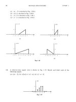
Figure
1.1.
Discrete-time signal
x[n]
Basic
Problems

(a). Define a
MATLAB
vector
nx
to be the time indices
-3
5
n
5
7
and the
MATLAB
vector
x
to be the values of the signal x[n] at those samples, where x[n] is given by
2,
n=O,
1,
n=2,
3,
n=4,
0, otherwise.
If
you have defined these vectors correctly, you should be able to plot this discrete-
time sequence by typing
stem(nx,x).
The resulting plot should match the plot shown
in Figure
1.1.
(b). For this part, you will define

MATLAB
vectors
yl
through
y4
to represent the follow-
ing discrete-time signals
Yl[nl
=
x[n
-
21,
ya[n]
=
x[n
+
11
7
~3[n]
=
x[ n]
,
y4[n]
=
x[-n
+
11
.
To do this, you should define
yl

through
y4
to be equal to
x.
The key is to define
correctly the corresponding index vectors
nyl
through
ny4.
First, you should figure
10
CHAPTER
1.
SIGNALS AND SYSTEMS
out how the index of
a
given sample of x[n] changes when transforming to yi[n]. The
index vectors need not span the same set of indices as
nx,
but they should all be at
least
11
samples long and include the indices of all nonzero samples of the associated
signal.
(c). Generate plots of
yl[n] through yr[n] using
stem.
Based on your plots, state how
each signal is related to the original
x[n], e.g., "delayed by

4"
or "flipped and then
advanced by
3."
1.4
Properties of Discrete-Time Systems
Discrete-time systems are often characterized in terms of a number of properties such as
linearity, time invariance, stability, causality, and invertibility. It is important to understand
how to demonstrate when a system does or does not satisfy a given property.
MATLAB
can be used to construct counter-examples demonstrating that certain properties are not
satisfied. In this exercise, you will obtain practice using
MATLAB to construct such counter-
examples fcr a variety of systems and properties.
Basic Problems
For these problems, you are told which property a given system does not satisfy, and the
input sequence or sequences that demonstrate clearly how the system violates the property.
For each system, define
MATLAB vectors representing the input(s) and output(s). Then,
make plots of these signals, and construct a well reasoned argument explaining how these
figures demonstrate that the system fails to satisfy the property in question.
(a). The system y [n]
=
sin((~/2)x[n]) is not linear. Use the signals xl [n]
=
6[n] and
xz[n]
=
26[n] to demonstrate how the system violates linearity.
(b).

The system y[n]
=
x[n]
+
x[n
+
11
is not causal.
Use the signal
x[n]
=
u[n] to
demonstrate this. Define the
MATLAB vectors
x
and
y
to represent the input on the
interval
-5
<
n
<
9,
and the output on the interval
-6
5
n
5
9,

respectively.
Intermediate Problems
For these problems, you will be given a system and a property that the system does not
satisfy, but must discover for yourself an input or pair of input signals to base your argument
upon. Again, create
MATLAB vectors to represent the inputs and outputs of the system
and generate appropriate plots with these vectors. Use your plots to make a clear and
concise argument about why the system does not satisfy the specified property.
(c). The system
y[n]
=
log(x[n]) is not stable.
(d). The system given in Part (a) is not invertible.
Advanced Problems
For each of the following systems, state whether or not the system is linear, time-invariant,
causal, stable, and invertible.
For each property you claim the system does not possess,
Sec.
1.5.
lrn~lementinn
a
First-Order Difference Equation
11
construct a counter-argument using MATLAB to demonstrate how the system violates the
property in question.
1.5
Implementing a First-Order Difference Equation
Discrete-time systems are often implemented with linear constant-coefficient difference equa-
tions. Two very simple difference equations are the first-order moving average
and the first-order autoregression

Even these simple systems can be used to model or approximate a number of practical
systems. For instance, the first-order autoregression can be used to model a bank account,
where
y[n] is the balance at time n, x[n] is the deposit or withdrawal at time n, and
a
=
l+r
is the compounding due to interest rate r. In this exercise, you will be asked to write a
function which implements the first-order autoregression equation. You will then be asked
to test and analyze your function on some example systems.
Advanced Problems
(a). Write a function
y=dif f eqn(a,x, yni)
which computes the output y[n] of the causal
system determined by Eq. (1.6). The input vector
x
contains x[n] for 0
5
n
5
N
-
1
and
ynl
supplies the value of y[-11. The output vector
y
contains y[n] for 0
5
n

<
N
-
1. The first line of your M-file should read
function y
=
diffeqn(a,x,ynl)
Hint: Note that y[-1] is necessary for computing y[O], which is the first step of the
autoregression. Use a
for
loop in your M-file to compute y[n] for successively larger
values of n, starting with n
=
0.
(b). Assume that
a
=
1, y[-1]
=
0, and that we are only interested in the output over the
interval
0
5
n
1
30. Use your function to compute the response due to xl[n]
=
6[n]
and x2[n]
=

u[n], the unit impulse and unit step, respectively. Plot each response
using
stem.
(c). Assume again that
a
=
1, but that y[-1]
=
-1. Use your function to compute y[n]
over 0
5
n
<
30 when the inputs are xl[n]
=
u[n] and x2[n]
=
2u[n]. Define the
outputs produced by the two signals to be
yl[n] and yz[n], respectively. Use
stem
to
display both outputs. Use
stem
to plot (2 yl[n]
-
y~[n]).
Given that Eq. (1.6) is a
linear difference equation, why isn't this difference identically zero?
12

CHAPTER
1.
SIGNALS AND SYSTEMS
(d). The causal systems described by
Eq.
(1.6) are BIB0 (bounded-input bounded-output)
stable whenever
la1
<
1.
A property of these stable systems is that the effect of
the initial condition becomes insignificant for sufficiently large
n.
Assume
a
=
112
and that
x
contains
x[n]
=
u[n]
for
0
<
n
5
30.
Assuming both

y[-1]
=
0
and
y[-1]
=
112, compute the two output signals
y[n]
for
0
5
n
5
30.
Use stem to display
both responses. How do they differ?
1.6
Continuous-Time Complex Exponential Signals
@
Before starting this exercise, you are strongly encouraged to work through the Symbolic
Math Toolbox tutorial contained in the manual for the Student Edition of
MATLAB. The
functions in the Symbolic Math Toolbox can be used to represent, manipulate, and analyze
continuous-time signals and systems symbolically rather than numerically. As
an example,
consider the continuous-time complex exponential signals which have the form
eSt,
where
s
is a complex scalar. Complex exponentials are particularly useful for analyzing signals and

systems, since they form the building blocks for a large class of signals. Two familiar signals
which can be expressed as a sum of complex exponentials are cosine and sine. Namely, by
setting
s
=
hiwt, we obtain
In this exercise, you will be asked to use the Symbolic Math Toolbox to represent some basic
complex exponential and sinusoidal signals. You will also plot these signals using ezplot,
the plotting routine of the Symbolic Math Toolbox.
Basic Problems
(a). Consider the continuous-time sinusoid
A symbolic expression can be created to represent
x(t) within MATLAB by executing
The variables of
x
are the single character strings
't
'
and
'TI.
The function ezplot
can be used to plot a symbolic expression which has only one variable, so you must
set the fundamental period of
x(t)
to a particular value. If you desire
T
=
5,
you can
use

subs
as follows
Thus
x5
is a symbolic expression for sin(2nt15). Create the symbolic expression
for
x5
and use ezplot to plot two periods of sin(2nt/5), beginning at
t
=
0.
If done
correctly, your plot should be as shown in Figure 1.2.
Sec.
1.6.
Continuous-Time Complex Exponential Signals
@
13
Figure
1.2.
Two periods of the signal sin(2nt/5)
(b). Create a symbolic expression for the signal
The two sinusoids should be created separately, and then combined using
symmul.
For
T
=
4,
8,
and

16,
use
ezplot
to plot the signal on the interval
0
5
t
5
32.
What is
the fundamental period of
x(t) in terms of
T?
Intermediate Problem
The response of some underdamped systems to an impulsive input can be modeled by
An example of a physical system which might generate such a signal is the sound generated
by striking a bell. This sound is well approximated by a single tone whose magnitude decays
with time. For underdamped systems, the
quality1
is often used to quantify the resonance of the system. The resonance is a measure of the
number of oscillations in the impulse response before the response effectively dies out. For
the bell example, the time at which the response dies out could be defined
as
the time at
which the sound becomes inaudible.
'The definition of quality in
Eq.
(1.9)
is actually an approximation of the quality defined in
Signals and

Systems
by Oppenheim and Willsky, and is valid only when
Ta
<<
n.
14
CHAPTER
1.
SIGNALS AND SYSTEMS
(c). Create a symbolic expression for the signal
For
a
=
112, 114, and 118, use
ezplot
to determine td, the time at which Ix(t)l
last crosses 0.1.
Define
td as the time at which the signal dies out. Use
ezplot
to
determine for each value of
a
how many complete periods of the cosine occur before
the signal dies out. Does the number periods appear to be proportional to
Q?
Advanced Problems
In the following problems you will write M-files for extracting the real and imaginary com-
ponents, or the magnitude and phase, of a symbolic expression for a complex signal.
(d). Store in

x
a syn~bolic expression for the signal
Remember to use
'
i
'
rather than
'
j
'
within symbolic expressions to represent
fl.
The function
ezplot
cannot be used directly for plotting x(t), since x(t) is a complex
signal. Instead, the real and imaginary components must be extracted and then
plotted separately.
(e). Write a function
xr=sreal(x)
which returns a symbolic expression
xr
representing
the real part of
x(t). If your function is working properly,
ezplot (xr)
will plot the
real component of
x(t). Similarly, write a function
xi=simag(x)
which returns

a
sym-
bolic expression
xi
representing the imaginary component of x(t). The first line of
the M-file
sreal .m
should be
function xr
=
sreal(x)
You can then use
compose
(
'real
(x)
'
,x)
to create a symbolic expression for the
real component of
x(t). Use
ezplot
and the functions you created to plot the real
and imaginary components of
x(t) on the interval 0
5
t
5
32. Use a separate plot for
each component. What is the fundamental period of

x(t)?
(f). For
x
containing the symbolic expression for x(t), create two functions
xm=sabs(x)
and
xa=sangle(x)
which create symbolic expressions representing the magnitude and
phase, respectively, of
x(t).
(g). Consider again x(t) as defined in Part (d). Use
ezplot
and the functions you created
to plot the magnitude and phase of
x(t) on the interval 0
5
t
5
32. Use separate plots
for the magnitude and phase. Why is the phase plot discontinuous?
1.7
Transformations of the Time Index for Continuous-Time Signals
@
This exercise will allow you to examine the effect of various transformations of the in-
dependent variable of continuous-time signals using
MATLAB's Symbolic Math Toolbox.
Sec.
1.7.
Transformations of the Time Index for Continuous-Time Sienals
@

15
Specifically, you will look at the effect of these transformations on a ramp-shaped pulse
signal
f
(t)
=
t(u(t)
-
'~l(t
-
2)),
(1.10)
where
u(t) is the unit step signal
The Symbolic Math Toolbox in the Student Edition of
MATLAB calls the unit step
function
Heaviside.
The function
ezplot
can only plot functions which are both in the
Symbolic Math and main
MATLAB toolboxes. Since
Heaviside
is only in the Symbolic
Math Toolbox, you will need to create an M-file called
Heaviside .m
in your working di-
rectory. The contents of this file are as follows
function f

=
Heaviside(t)
%
HEAVISIDE Unit Step function
%
f
=
Heaviside(t1 returns a vector
f
the same size as
%
the input vector, where each element of f is
1
if the
%
corresponding element of t is greater than or equal to
%
zero.
f
=
(t>=O);
If you have defined this function properly, you should be able to duplicate the following
example
>>
Heaviside([-l:0.2:1])
ans
=
0 0 0
0
0

1
1
1
1
1 I
Intermediate Problems
(a). Use
Heaviside
to define
f
to be a symbolic expression for
f
(t)
as
specified in Eq. (1.10).
Plot this symbolic expression using
ezplot.
(b). The expressions below define a set of continuous-time signals in terms off (t). For each
of the following signals, state how you expect it to be related to
f
(t), e.g., "delayed
by
7,"
"flipped then advanced by 16":
16
CHAPTER
1.
SIGNALS AND SYSTEMS
(c). Use the Symbolic Math Toolbox function
subs

and the symbolic expression
f
you
defined in Part (a) to define symbolic expressions in
MATLAB called
gl
through
g5
to represent the signals in Part (b). Plot each signal using
ezplot
and state whether
or not the plot agrees with your prediction from Part (b).
1.8
Energy and Power for Continuous-Time Signals
@
For a continuous-time signal x(t), the energy over the interval -a
5
t
<
a is often defined
as
where (xI2
=
xx* and x* is the complex conjugate of x. Thus, for a periodic signal with
fundamental period
T,
ET12
contains the signal energy over one period. The energy in the
entire signal is defined
as

Em
=
lim
Ea
,
a+w
if the limit exists. While most signals in practice have finite energy, many of the continuous-
time signals used
as
conceptual tools for signals and systems do not. For example, any
periodic signal has infinite energy. For these signals, a more useful measure is average
power, which is simply energy divided by the length of the time interval. Thus, the time-
average power over the interval -a
<
t
<
a is
En
a>O,
and the time-average power of the entire signal is
Pw
=
lim
Pa,
a+w
if the limit exists. In this problem, you will consider how
P,
and
ETI2
are related for

periodic signals.
Basic Problems
(a). Create symbolic expressions for each of the following three signals
x,(t)
=
cos(7rt/5)
,
xz (t)
=
sin(~t/5)
,
x3(t)
=
e
i2nt.13
+
ei~t
These expressions will have
't'
as
a
variable. You might want to use the function
symadd
when creating the symbolic expression for x3(t).
(b). Use
ezplot
to plot two periods of each signal. If the signal is complex, be sure to
plot the real and imaginary components separately. The axes of your plots should
be appropriately labeled. Hint: You can extract the real component of
a

symbolic
expression using
compose('real(x)' ,x).
If you have done Exercise
1.6,
use the
functions you created there.