NUMERICAL SIMULATIONS EXAMPLES AND APPLICATIONS IN COMPUTATIONAL FLUID DYNAMICS_2 pptx

11
Comparison of Numerical Simulations and
Ultrasonography Measurements of the Blood
Flow through Vertebral Arteries
Damian Obidowski and Krzysztof Jozwik
Technical University of Lodz,
Institute of Turbomachinery, Medical Apparatus Division
Poland
1. Introduction
Vertebral arteries are a system of two blood vessels through which blood is carried to the
rear region of the brain. This region of the human body has to be very well supplied with
blood. Blood is delivered to the brain through carotid arteries as well. Due to their position
and shape, vertebral arteries are a special kind of blood vessels. They have their origin at a
various distance from the aortic ostium, can branch off at different angles, and have various
lengths, inner diameters and spatial shapes. The above-mentioned variations are connected
with inter-patient differences in the human anatomy. In the upper part of vertebral arteries,
there is a marked arch curvature, owing to which turning the head is not followed by
obliteration of these vessels. Contrary to other arteries, vertebral arteries join at their ends to
form one vessel, a comparatively large basilar artery. This junction can be characterized by a
varied geometry as well. For individual geometrical configurations of the vertebral artery
system, there are also differences in the diameter of the left and right artery. All the above-
mentioned differences result from a unique individual anatomical structure and do not
follow from any pathology (Daseler & Anson 1959; Jozwik & Obidowski 2008; Jozwik &
Obidowski 2010).
Some symptoms occurring in patients may suggest that the cause of an ailment lies in an
incorrect blood supply to the rear region of the brain, and thus in an incorrect blood flow
through vertebral arteries. The direct cause of such a phenomenon can result from arterial
occlusion. The ultrasonography is employed to check the flow correctness. It is rather
difficult to conduct this imaging procedure, but if it is performed by an experienced
specialist, then the results obtained can be considered reliable. It happens, however, that the
measured values of the maximum and minimum velocity in the left and right artery, which

characterize the blood flow, differ significantly. Hence, the diagnosis of arteriosclerosis in
these vessels is well based. It can be an indication for a surgical procedure (Mysior 2006). A
significantly large percentage of cases diagnosed in such a way are not related to changes in
the artery structure, and thus surgery would be irrelevant. If a structure and a shape of
vertebral arteries, their individual variations are considered, then differences in the blood
flow and a lack of relation between these differences and artery diameters can result from
flow phenomena only.
Numerical Simulations - Examples and Applications in Computational Fluid Dynamics

214
The aim of the present study is to investigate the hydrodynamics of the blood flow through
three different kinds of artery geometries to have a better insight into the phenomena
occurring in the human body and to compare these simulation results with results of
ultrasonography measurements (Jozwik & Obidowski 2008, Jozwik & Obidowski 2010).
2. Structure of vertebral arteries
In the human anatomical structure, several basic types of the spatial geometry in vertebral
arteries can be differentiated. A frequency of their occurrence varies and one can say that
three or four of them at most refer to the majority of cases met. Figure 1 presents types of the
geometrical structure of vertebral arteries and a percentage of their occurrence in
population.


Fig. 1. Types of the vertebral artery structure and a percentage of their occurrence in
population: a) the most frequently appearing case, b) the left artery starting significantly
below, c) the right artery starting from the point far from the origin of carotid arteries, d) the
left artery starting from the aortic arch, e, f, g) other structures resulting in less than 1% cases
(Daseler & Anson 1959)
An essential aspect of the structure of vertebral arteries is their 3D characteristic curve. For a
given type of the vertebral artery structure, there occur differences, often significant, in
Comparison of Numerical Simulations and Ultrasonography Measurements

of the Blood Flow through Vertebral Arteries

215
inner diameters (left to right and patient to patient), and thus in flow fields. Such variations
in inner diameters do not exceed the range of 2 – 6 mm. However, for a particular patient
anatomy, the inner diameter, except for stenosis occurring in arteries, of an individual
vertebral artery can be treated as constant along the artery. Nevertheless, it is impossible to
formulate explicit relations describing the dependence between the left and right artery
inner diameter. Each configuration of diameters (whose values fall within the range
mentioned) is possible (Daseler & Anson 1959; Sokołowska 1988).
3. Model of the selected structure geometry
For the system of the vertebral artery structure occurring most frequently in the human
anatomical structure, three models of its geometry have been developed (see Fig. 2). Each
model has one inlet (aortic ostium) and six outlets (cross-sections of main arteries in the
considered region). Owing to a significant differentiation in individual human anatomy
(Daseler and Anson 1959; Ravensbergen et al.1974), which consists in a varied arrangement,
length, kind of junctions, inner diameters and other geometrical parameters of the blood
vessels under consideration, averaged data included in anatomical atlases, scientific
publications, results of tomographic, magnetic resonance and ultrasonography imaging
(Daseler and Anson 1959; Bochenek and Reicher 1974; Daniel 1988; Michajlik and
Ramotowski 1996; Sinelnikov 1989; Vajda 1989) have been employed in the models
developed. The models of vertebral arteries do not account for a part of secondary vessels
branching off from the arteries under analysis before they join to form the basilar artery.
Diameters of these vessels are relatively very small and their effect on the flow is
insignificant.


Fig. 2. Developed models of the selected geometry of the vertebral artery region of the
circulatory system (Obidowski 2007)
The 3D shape of arteries has been taken into account in the three models prepared. These

models differ as far as the place the left and right artery starts, the spatial shape and the
length of individual arteries are concerned. For each model further on referred to as model
1, 2 and 3, differences in the total length of the left and right artery occur that are equal to,
respectively: for model 1 – left artery – 501.8 mm, right artery – 522.8 mm, for model 2 – left
artery – 501.8 mm, right artery – 502.8 mm, for model 3 – left artery – 466.3 mm, right artery
a
) b) c)
Numerical Simulations - Examples and Applications in Computational Fluid Dynamics

216
– 522.8 mm. These differences result from various places the left or right vertebral artery
originates. Model 3, in which the left artery starts directly on the aortic arch, differs mostly.
Moreover, it has been assumed that artery diameters can vary within the range of the values
quoted above, but they are constant along their length. Taking into consideration changes in
the inner diameter with a step equal to 1 mm and the fact that an arbitrary combination of
the left and right artery diameter can occur, 25 cases of geometry for each model system and
three different system geometries have been obtained, giving altogether 75 cases to be
analysed. To simulate the flow, walls of all vessels considered have been assumed rigid and
not subject to deformations with changes in the blood pressure. The diameters of the
remaining artery vessels in the segments under consideration are listed in Table 1.

Artery Diameter [mm]
Aorta 28.5
Brachiocephalic trunk artery 20 at bifurcation ÷ 14 at the outlet cross-section
Right carotid artery 14 at bifurcation ÷ 12 at the outlet cross-section
Left carotid artery 12 at bifurcation ÷ 11.5 at the outlet cross-section
Left subclavian artery 16 at bifurcation ÷ 15.5 at the outlet cross-section
Basilar artery 3 ÷ 8.5 depending on the vertebral artery diameter
Vertebral arteries 2 ÷ 6 depending on the case studied
Table 1. Values of diameters used to model the geometry (Bochenek 1974; Daniel 1988;

Mysior 2006; Vajda 1989 et al.)
For each case of the system geometry, a computational mesh built of tetrahedral elements,
condensed in the region of vertebral arteries, has been generated. Additionally, prism
elements have been introduced in the vicinity of walls to define flow parameters at vessel
walls more precisely. A sample mesh can be found in (Obidowski 2007, Jozwik and
Obidowski 2010). The mesh independence tests have not yielded any significant differences
that could affect the results of the computations conducted. Thus, due to time-consuming
transient simulations, a middle-size density has been employed. The average size of the
mesh used is approx. 1 million elements.
4. Blood flow parameters and boundary conditions
Blood is the medium owing to which each place in our organism is supplied with products
indispensable for life and simultaneously purified from waste or toxic substances. From the
viewpoint of flow, blood parameters are very difficult to describe. Even for a particular
individual, values of the parameters alter, and these alterations depend on numerous factors
connected with sex, age, diet and physical conditions, etc. Moreover, variations in values of
blood flow parameters occur both slowly (e.g., along with the patient’s ageing), as well as
very fast (e.g., as an effect of irritation). The blood flow in human body is a cyclic flow with
a strong asymmetry of changes within one cycle. In addition, owing to damping properties
of blood vessel walls, amplitude and pressure variations versus time undergo changes
depending on a position and a distance of the point under consideration from the heart. A
proper model of blood, as well as properly imposed boundary conditions exert a direct
Comparison of Numerical Simulations and Ultrasonography Measurements
of the Blood Flow through Vertebral Arteries

217
influence on the quality and accuracy of computations (Ballyk et al. 1994; Chen & Lu 2006;
Gijsen et al. 1999; Johnston et al. 2004; Obidowski 2007, Walburn & Schneck 1976). On the
other hand, taking into account a relatively wide range of alternations in values of these
parameters, the blood model should reflect its behaviour in the flow and not necessarily
render exactly the values of individual quantities that describe blood flow characteristics.

4.1 Model of blood
From the viewpoint of flow, the fundamental blood parameters are as follows:
- density,
- viscosity,
- heat conductivity.
For the phenomena and the region under consideration, the last parameter can be neglected.
Changes in blood density depend on age and sex of the person first of all and their values
fall within the range of 1030 – 1070 kg/m
3
(Bochenek et al. 1974, Michajlik et al. 1996). For
the needs of this simulation, the constant density of blood equal to 1055 kg/m
3
has been
assumed.


Fig. 3. Apparent blood viscosity as a function of strain for different blood models (Johnston
et al. 2004)
Blood is a non-Newtonian fluid with a state memory. It means that the dynamic viscosity
coefficient does not depend on the kind of liquid only, but also on flow parameters and a
tendency in their variations. In the literature, numerous models describing a relation
between the blood viscosity coefficient and blood flow parameters can be found. To describe
Numerical Simulations - Examples and Applications in Computational Fluid Dynamics

218
the flow occurring in vicinity of the aortic ostium, the Newton’s model is appropriate. On
the other hand, the blood flow in small vessels needs a more complex blood model (Ballyk
et al. 1994; Chen and Lu 2006; Gijsen et al. 1999; Johnston et al. 2004; Obidowski 2007,
Walburn and Schneck 1976). For the purpose of this study, a modified Power Law model
has been employed. This model reflects the behaviour of the Newtonian fluid for large

Reynolds numbers and simultaneously renders the flow nature at the viscosity of blood
vessels of low diameters and low velocities. The model is expressed by the following system
of equations:

1
2
9
i
ij
j
n1
11
22
9
ii
0ij ij
jj
1
2
i
ij
j
U
μ 0.554712 for 2 S 1e
x
UU
μμ 2 S for 1e 2 S 327
xx
U
μ 0.00345 for 2 S 327

x
−
−
−
⎧
⎛⎞
∂
⎪
=<
⎜⎟
⎪
⎜⎟
∂
⎝⎠
⎪
⎪
⎛⎞
⎪
⎛⎞ ⎛⎞
⎜⎟
∂∂
⎪
=≤<
⎜⎟ ⎜⎟
⎨
⎜⎟
⎜⎟ ⎜⎟
∂∂
⎪
⎝⎠ ⎝⎠

⎜⎟
⎝⎠
⎪
⎪
⎛⎞
⎪
∂
=≥
⎜⎟
⎪
⎜⎟
∂
⎪
⎝⎠
⎩
(1)
where: = 0.0035 Pa s, n = 0.6 and
1
2
i
ij
j
U
2S
x
⎛⎞
∂
⎜⎟
⎜⎟
∂

⎝⎠
- shear strain rate.
Characteristic curves as a function of strain are presented in Fig. 3. The same curves show
variations in other blood models known from the literature (Johnston et al. 2004; Gijsen et al.
1999; Walburn & Schneck 1976).
4.2 Boundary conditions
For the system under consideration, boundary conditions referring to time-variable
parameters at the inlet and in six outlet cross-sections (see Fig. 4) should be assumed.
Velocity variations versus time, as well as pressure variations can be approximated with a
Fourier series. The Fourier series employed to determine the velocity and pressure waves
takes the following form:

() ()()
()
3
0n 0n 0
n1
1
Ft a acosn t t bsinn t t
2
ωω
=
=+ ++ +
∑
(2)
where a
0
, a
n
and b

n
are experimentally determined Fourier coefficients and t
0
is a phase
displacement. Thus, at the inlet, that is to say, at the aortic ostium, a uniform velocity
distribution for the whole cross-section has been adopted. Six harmonics of the Fourier
series allow one to generate a velocity profile used in the presented experiment as shown in
Fig. 5, which is an approximation of experimental curves found in the literature (Traczyk
1980, Viedma 1997).
The time-variable static pressure has been taken as the parameter determining boundary
conditions at outlets. The static pressure also changes periodically and a time displacement
of these changes following from various paths of the pulse wave measured from the aortic
Comparison of Numerical Simulations and Ultrasonography Measurements
of the Blood Flow through Vertebral Arteries

219
ostium should be taken into account for the assumed outlet cross-sections. The values of
phase displacements for individual outlet cross-sections have been calculated on the basis of
the length of centre lines and pulse wave propagation velocities in arteries. Wang has
determined pulse wave propagation velocities in individual human arteries (Wang 2004).
For the outlet cross-section of the basilar artery, the pressure has been determined on the
basis of the averaged path along the left and right vertebral artery. The static pressure
variations for individual outlets are shown in Fig. 6 (Jozwik & Obidowski 2009).


Fig. 4. Boundary conditions at the inlet and outlets of the modelled geometry of the
vertebral arteries under investigation (Obidowski 2007)
The walls of vessels in which blood flows are supposed to be nondeformable. Owing to the
flow nonstationarity that follows both from considerable values of velocity at the aortic
ostium, numerous branches and narrowings, as well as from a pulsating nature of the flow,

the flow is expected to be turbulent in many places of the system being modelled. A Shear
Stress Transport (SST) model, belonging to the k-ω model family, has been adopted as the
turbulence model in the investigations.
This model renders correctly the character of the boundary flow for the flows characterized
by low Reynolds numbers. Initially, the calculations were conducted for the flow under
steady conditions.
Numerical Simulations - Examples and Applications in Computational Fluid Dynamics

220

Fig. 5. Changes in velocity as a function of time for the inlet cross-section during one cycle of
heart operation (Obidowski 2007)


Fig. 6. Changes in pressure as a function of time for outlet cross-sections during one cycle of
heart operation (Jozwik & Obidowski 2009)
Comparison of Numerical Simulations and Ultrasonography Measurements
of the Blood Flow through Vertebral Arteries

221
The following values of parameters at the inlet and the outlet were taken, namely:
-
velocity in the aortic ostium, v
as
= 1.44 m/s,
-
all static pressures in all outlet cross-sections were assigned to averaged static pressures
and were equal to 13 kPa.
The results obtained for steady flow calculations were taken as the initial ones for the
unsteady flow, for which the calculations of five cycles of variations in parameters were

conducted. Owing to this, the obtained results are independent of the assumed initial values
from the steady flow conditions.
4.3 Governing equations
The ANSYS CFX v. 10.0 solver was used to obtain a solution to the described problem. The
unsteady Navier-Stokes equations in their conservation form are a set of equations solved
by ANSYS CFX (ANSYS CFX-Solver Theory Guide).
The continuity equation is expressed as:

()
ρ
ρU0
t
∂
+
∇⋅ =
∂
(3)
Thus, the momentum equation takes the following form:

(
)
()
M
ρU
ρUU p τ S
t
∂
+∇⋅ ∗ =−∇ +∇⋅ +
∂
(4)

where the stress tensor,
τ
, is related to the strain rate by the following relation:

()
T
2
τμ UU δ U
3
⎛⎞
=
∇+∇ − ∇⋅
⎜⎟
⎝⎠
(5)
The total energy equation is represented by:

(
)
()()()
tot
tot M E
ρh
p
ρUh λ TUτ US S
tt
∂
∂
−
+∇⋅ =∇⋅ ∇ +∇⋅ ⋅ + ⋅ +

∂∂
(6)
where h
tot
is the total enthalpy, related to the static enthalpy h(T, p) by:

2
tot
1
hhU
2
=+
(7)
The term
∇⋅(U⋅τ) represents the work due to viscous stresses and is called the viscous work
term. The term U
⋅S
M
refers to the work due to external momentum sources and is currently
neglected.
An alternative form of the energy equation, which is suitable for low-velocity flows, is also
available. To derive it, an equation for the mechanical energy K is required. This equation
has the form:

2
1
KU
2
=
(8)

The mechanical energy equation is derived by taking the dot product of U with the
momentum equation:
Numerical Simulations - Examples and Applications in Computational Fluid Dynamics

222

()
() ()
M
ρK
ρUK U p U τ US
t
∂
+∇⋅ =− ⋅∇ + ⋅ ∇⋅ + ⋅
∂
(9)
In the present paper, the thermal energy equation is not taken into consideration as the
blood flow in the short time is isothermal, thus energy dissipation and heat conductivity is
neglected.
5. Results
For the 75 model geometrical cases investigated that cover changes in inner diameters of
vertebral arteries of the three selected types of their spatial geometry, the results that allow
for an analysis of velocity distributions during the whole cycle of heart operation in an
arbitrary point of the modelled system have been obtained. The distance of the origin of
vertebral arteries from the aortic ostium enables one to determine proper velocity profiles at
the points crucial from the viewpoint of the investigations conducted. As an example,
velocity profiles determined in the left and right vertebral artery during the first phase of
the simulated cycle of heart operation (range of 0.15 – 0.30 s) are depicted in Fig. 7. One can
see the velocity profile that suggests a laminar flow for small diameters, whereas for large
diameters of blood vessels, the obtained profiles are deformed by unsteadiness of the

phenomena and an effect of the duct curvature can be observed.
Determination of the flow structure versus time at the point where vertebral arteries join to
form the basilar artery is more important for the investigation. Figures 8 and 9 show various
velocity profiles in this point for five time instants of the heart operation cycle for the
selected geometrical variants of three modelled structures and two different diameters of
left and right arteries (Fig. 8 shows distributions for the diameter of the left artery equal to 3
mm and the right one – 5 mm and Fig. 9 presents the different situation – the diameter of the
left artery equals 4 mm and of the right one – 2 mm). A very strong disproportion of the
velocity of blood flowing into the basilar artery from the left and right artery and between
the same arteries in different models can be observed. Of course, the result obtained refers to
the selected geometry and is not characteristic of all cases under consideration. A possibility
to compare changes in velocity of the left and right artery during one cycle of heart
operation for the three selected geometries and three modelled structures of vertebral
arteries is provided by the distributions shown in Fig. 10.
An effect of the velocity increase cannot be observed in the artery with an increasing
diameter. Even for the identical diameter of both arteries, the velocity profile differs
significantly. For the constant diameter of the arteries, both the left and the right one (see
Fig. 10 b and c), a change in the diameter of the second artery affects differently a change in
the velocity in the artery under consideration. In the left vertebral artery, the maximum
velocity is attained for the same diameter of both the arteries (4 mm), whereas for the right
artery, such behaviour was observed for the largest diameter of the left artery (6 mm). In this
case, differences between the velocities occurring for individual diameters of the left artery
under analysis are considerably lower. For the given low, constant diameter of the left artery
equal to 2 mm (see Fig. 10 a), the maximum velocity occurs for two values of the right artery
diameter (4 and 6 mm). Here, for the diameter of the right artery equal to 5 mm, a sharp
decrease in the maximum velocity value in the left artery occurs. An effect of wave
phenomena on the flow in arteries can be clearly seen.
Comparison of Numerical Simulations and Ultrasonography Measurements
of the Blood Flow through Vertebral Arteries

223

Fig. 7. Velocity distribution along the diameter of the left and right vertebral artery for one
geometrical configuration at different instants of the heart operation cycle (t = 0.15 s, t = 0.2
s, t = 0.25 s, t = 0.3 s) (Obidowski 2007)
Some possibilities to compare the effect of diameters of the left and right vertebral artery on
the values of velocity, which were obtained in these blood vessels during the simulations,
are provided by a comparison of maximum velocities within the single heart cycle,
measured in the centre part of the left and right artery for all the diameter configurations
and for three modelled structures of these vessels analysed. This comparison is presented in
Fig. 11 but only for the changes in the diameter from 2 to 5 mm as data from
ultrasonography measurements were available only for this range. Moreover, the values of
the maximum velocity for the defined diameters corresponding to the vessel diameters,
calculated on the basis of the Hagen-Poiseuille equation, are shown. The equation is
frequently used in medicine to compare the velocities in both the arteries (left and right) on
the basis of the resistance assumed in vessels being a function of their diameters and a
pressure drop in vertebral arteries.
Numerical Simulations - Examples and Applications in Computational Fluid Dynamics

224
Model 1 Model 2 Model 3
t = 0.10t = 0.15t = 0.20t = 0.25t = 0.30

Fig. 8. Comparison of velocity profiles at the point vertebral arteries join to form the basilar
artery for three spatial geometrical variants of the same diameter variant (left3right5) and
for five time instants of the heart operation cycle (t = 0.1 s, t = 0.15 s, t = 0.2 s, t = 0.25 s,
t = 0.3 s)
Comparison of Numerical Simulations and Ultrasonography Measurements
of the Blood Flow through Vertebral Arteries

225
Model 1 Model 2 Model 3
t = 0.10t = 0.15t = 0.20t = 0.25t = 0.30

Fig. 9. Comparison of velocity profiles at the point vertebral arteries join to form the basilar
artery for three spatial geometrical variants of the same diameter variant (left4right2) and
for five time instants of the heart operation cycle (t = 0.1 s, t = 0.15 s, t = 0.2 s, t = 0.25 s,
t = 0.3 s)
Numerical Simulations - Examples and Applications in Computational Fluid Dynamics

226



Fig. 10. Velocity distributions vs. time for one heart operation cycle in the left and right
vertebral artery for three geometrical variants of blood vessels (left 2 mm, right 4 mm, left
6 mm) (Obidowski 2007)
a
)
b)
c)
Comparison of Numerical Simulations and Ultrasonography Measurements
of the Blood Flow through Vertebral Arteries

227


0
0.1
0.2

0.3
0.4
0.5
0.6
0.7
0.8
0.9
1
Velocity [m/s]
Comparison of peak systolic velocities for the left vertebral artery
V max USG
V max model1
V max model2
V max model3
according to the Hagen-Poiseuille’s equation


0
0.1
0.2
0.3
0.4
0.5
0.6
0.7
0.8
0.9
1
Velocity [m/s]
Comparison of peak systolic velocities for the right vertebral artery

V max USG
V max model1
V max model2
V max model3
according to the Hagen-Poiseuille’s equation

Fig. 11. Comparison of the maximum value of velocities obtained for the left and right
vertebral artery for all investigated geometrical configurations of the system,
ultrasonography measurements and calculated on the basis of the Hagen-Poiseuille
equation (Obidowski 2007)
b)
a)
Numerical Simulations - Examples and Applications in Computational Fluid Dynamics

228
The same plot shows the maximum velocity values obtained from ultrasonography
measurements in 520 people. The results have been averaged for all patients who had
individual values of diameters of vertebral arteries, but without distinguishing the type of
the spatial structure of arteries (Mysior 2006).
A good conformity between the results obtained from simulations and measurements
(without distinguishing the type of geometry of arteries) occurs in the central region, which
means a lack of conformity at the smallest diameters and for the two largest diameters. In
case of large vertebral artery diameters, the results of measurements agree with those
obtained on the basis of the Hagen-Poiseuille equation. For large diameters, an undisturbed
laminar flow occurs, and thus the above-mentioned equation, which refers basically to such
flows, yields correct results. A difference in the simulation results can follow from the fact
that artery wall deformations have not been considered. It also refers to the case of the
variant with the smallest diameters where the simulation results do not agree with the
measurements. The vessel wall material is not subject to the Hook’s law, and the
relationship between the deformation and the pressure inside the vessel (or, strictly

speaking, a difference in pressure between its inside and outside) is strongly nonlinear and
dependent on the individual human anatomical structure. Thus, modelling the
deformations in vertebral artery walls as a function of the flowing blood is extremely
difficult if not impossible at all.
6. Discussion
The conducted numerical investigations confirm a possibility of modelling the geometry of the
system of vertebral arteries together with vessels in their vicinity and of obtaining results that
enable an analysis of the effect of an artery diameter on velocity distributions in vessels during
the heart operation cycle for the selected, determined type of spatial geometry. The results
obtained indicate explicitly that differences in the flow and instantaneous velocity values in
vertebral arteries and in the point they join to form the basilar artery may not result from
pathological changes in the artery system, but can follow from physical phenomena that occur
in arteries as a consequence of the pulsating character of flow and the unique geometry, which
is related to the individual human anatomical structure.
The presented results refer to selected models of the vertebral artery structure and do not
account for changes in the length of individual arteries. Taking into account such a
possibility of changes within one model of the system (not only vessel diameters are
variable, but their length as well), the determination of the cause of disproportions found in
the flow in vertebral arteries is very difficult and complex.
The maximum velocity in one vertebral artery is affected by the flow in the other one (see
Fig. 11), thus the flow in the basilar artery strongly depends on the diameters and lengths of
both vertebral arteries.
The results of calculations according to the Hagen-Poiseuille equation, commonly used in
medicine for determination of the relation between flows in vertebral arteries, do not allow
one even to predict the behaviour of the flow. All properties of the flow in such arteries are
against the assumptions of the flow described by the above-mentioned equation. It is clearly
visible that the results obtained in the presented investigations differ significantly from
those calculated according to the Hagen-Poiseuille equation (see Fig. 11).
While analysing the obtained results, one should remember about the fact that rigid walls of
vessels have been assumed. This assumption affects directly the lack of energy accumulation

Comparison of Numerical Simulations and Ultrasonography Measurements
of the Blood Flow through Vertebral Arteries

229
during the cardiac contraction phase and its recovery during the heart relaxation. Moreover,
rigid vessels do not cause damping of the phenomena occurring during the flow in vertebral
arteries. Taking into account deformability of vessel walls through an introduction of their
rigidity, it will be possible to obtain a better approximation. An influence of flexible walls of
arteries should be especially observed in the values of minimum velocities of blood and in
obtaining reverse flows in vertebral arteries. An influence of the brain supply by carotid
arteries should be taken into account, as only completeness of the system will allow one to
consider a possibility of occurrence of wave phenomena. As a result, these phenomena can
be proven to follow from the pulsating flow and the vessel geometry.
In order to evaluate the simulation results, a model of the actual system of vessels for the
selected patient should be developed. Flows in vertebral arteries and blood systolic and
diastolic pressure should be measured for the selected geometry and, on this basis, the
boundary and initial conditions for the simulation should be defined. Only thus prepared
models and data will enable a correlation of the results of calculations and measurements.
7. Notations
,σ,σ,ββ,α,
k
'
ϖ
– constants,
k
– turbulence kinetic energy,
ω
- turbulence frequency,
μ
- dynamic viscosity,

t
μ - turbulence viscosity,
U
- velocity vector,
ρ
- density,
t
ν - eddy viscosity,
S
- invariant measure of the strain rate,
t
P - turbulence production due to viscous and buoyancy forces.
8. References
Ballyk P.D., Steinman D.A. & Ethier C.R. (1994). Simulation of non-Newtonian blood flow in
an end-to-end anastomosis,
J. Biorheology Vol., No., 31, pp. 565–586.
Bochenek A. & Reicher M. (1974).
Human anatomy, volume III, PZWL, ed. V, Warsaw, (in
Polish).
Chen J. & Lu X.Y., (2006). Numerical investigation of the non-Newtonian pulsatile blood
flow in a bifurcation model with a non-planar branch,
J. Biomechanics, Vol., No., 39,
pp. 818 – 832.
Daniel B., (1988).
Atlas of human radiological anatomy, PZWL, Warsaw, (in Polish).
Daseler E. H. & Anson B. J., (1959). Surgical anatomy of the subclavian artery and its
branches,
Surgery, Gynecology & Obstetrics, pp. 149-174.
Gijsen, F.J.H., van de Vosse, F.N. & Janssen, J.D. (1999). The Influence of the Non-Newtonian
Properties of Blood on the Flow in Large Arteries: Steady Flow in a Carotid

Bifurcation Model,
J. Biomechanics Vol., No., 32, pp. 601–608.
Numerical Simulations - Examples and Applications in Computational Fluid Dynamics

230
Gijsen, F. J. H., Allanic, E., van de Vosse, F. N., & Janssen, J. D., (1999). The Influence of the
Non-Newtonian Properties of Blood on the Flow in Large Arteries: Unsteady Flow
in a 90° Curved Tube,
J. Biomechanics, Vol., No., 32, pp. 705–713.
Johnston B. M., Johnston P. R., Corney S. & Kilpatrick D. (2004). Non-Newtonian blood flow
in human right coronary arteries: steady state simulations,
J. Biomechanics Vol. No.,
37, pp. 709-720.
Jozwik K. & Obidowski D., (2008). Geometrical models of vertebral arteries and numerical
simulations of the blood flow through them,
Proceedings of BioMed2008, 3rd Frontiers
in Biomedical Devices Conference & Exhibition
, pp. 5., BioMed2008-38048, ISBN 0-
7918-3823-4, Irvine, California, USA, June 2008, ASME.
Jozwik K. & Obidowski D., (2009). Numerical simulations of the blood flow through
vertebral arteries.
J. Biomechanics, Vol., No., 43, pp. 177-185.
Michajlik A. & Ramotowski W. (1996).
Human anatomy and physiology, PZWL, pp. 354-356 (in
Polish).
Mysior M., (2006).
Doppler ultrasound criteria of physiological flow in asymmetrical vertebral
arteries
, PhD Thesis, Polish Mother Memorial Research Institute, Lodz, 2006 (in
Polish).

Obidowski D., (2007).
Blood flow simulation in human vertebral arteries, PhD Thesis, Technical
University of Lodz, Lodz, 2007 (in Polish).
Obidowski D., Mysior M., Jozwik K., (2008). Comparison of Ultrasonic Measurements and
Numerical Simulation Results of the Flow through Vertebral Arteries,
Proceedings of
4th Conference of the International Federation for Medical and Biological Engineering, pp.
23-27, Belgium, Antwerp, November 2008, IFMBE Vol. 22, pp. 286-292, Springer-
Verlag Berlin, Heidelberg, 2009.
Ravensbergen J., Krijger J.K.B., Hillen B., Hoogstraten H.W. (1996). The Influence of the
Angle of Confluence on the Flow in a Vertebro-Basilar Junction Model.
J. Biomechanics, Vol., No., 29, pp. 281-299
Sinelnikov R.D., (1989).
Atlas of human anatomy, Mir Publishers, Moscow.
Sokołowska J. - Pituchowa (eds.), (1988).
Human anatomy, PZWL, Warsaw, (in Polish).
Traczyk W., Trzebski A., (1980).
Human physiology with elements of clinical physiology, PZWL,
Warsaw 1980 (in Polish).
Vajda J., (1989).
Atlas of human anatomy, Akademia Kiodo, Budapest (in Polish).
Viedma A., Jimenez-Ortiz C. & Marco V., (1997). Extended Willis circle model to explain
clinical observations in periorbital arterial flow.
J. Biomechanics, Vol., No., 30, pp.
265-272.
Wang J.J. & Parker K.H. (2004). Wave propagation in a model of the arterial circulation.
J. Biomechanics, Vol., No., 37, pp. 457-470.
Walburn, F.J. & Schneck, D.J. (1976). A constitutive equation for whole human blood.
Biorheology Vol., No., 31, pp. 201-218.

12
Numerical Simulation of Industrial Flows
Hernan Tinoco
1
, Hans Lindqvist
1
and Wiktor Frid
2

1
Forsmarks Kraftgrupp AB,
2
Swedish Radiation Safety Authority
Sweden
1. Introduction
Computational Fluid Dynamics (CFD) is a numerical methodology for analyzing flow
systems that may involve heat transfer, chemical reactions and other related phenomena.
This approach employs numerical methods imbedded in algorithms to solve general
conservation and constitutive equations together with specific models within a large
number of control volumes (cells or elements) into which the associated computational
domain of the flow system has been divided to build up a grid.
Numerical simulation of industrial flows using commercial CFD codes is now well
developed in a number of technical fields. With the advent of powerful and low-cost
computer clusters, events including both complex geometry and high Reynolds numbers,
i.e. fully turbulent practical industrial applications, may today be accurately modeled. This
technique constitutes a rather new tool for analyzing problems related to, for instance,
design, performance, safety and trouble-shooting of industrial systems since time can now
be treated fully as the primary independent variable.
The first commercial general-purpose CFD code, built around a finite volume solver, the
Parabolic Hyperbolic Or Elliptic Numerical Integration Code Series (PHOENICS), was

released in 1981. Initially, the solver was conformed to work only with structured, mono-
block, regular Cartesian grids but it was subsequently broadened to admit even structured
body-fitted grids. The multi-block grid option was developed many years later within this
code which still preserves this restricting structured grid topology. Another well known
commercial CFD code, FLUENT, was brought out onto the market in 1983 as a structured
software that bore a resemblance to PHOENICS, but aimed towards modeling of systems
with chemical reactions, specifically those related to combustion.
Hence, during the 1980s, CFD simulations were limited to rough time-independent models
with very simplified geometry due to the grid-structured character of the software and the
vast limitations in, at that time, normally available computer resources at the industry (see
e.g. Tinoco & Hemström, 1990). It might be of some interest to point out that the top
performance of a supercomputer at the end of the 1980s was of the order of 10 GFLOPS
(10×10
9
FLoating point Operations Per Second). The computers normally available at the
industry had a thousandth to a hundredth of that performance, i.e. 10-100 MFLOPS. Today,
a computer cluster containing a couple of hundred CPUs has a capacity of the order of
TFLOPS.
At the beginning of the 1990s, important steps in software improvement took place through
the development of grid-unstructured, parallelized algorithms (e.g. FLUENT UNS) that
Numerical Simulations - Examples and Applications in Computational Fluid Dynamics

232
enabled the possibility of an accurate geometrical representation of the modeled flow
system (see e.g. Tinoco & Einarsson, 1997). At the same time, the communication through
adequately formatted geometrical data between grid generators and CAD solid modelers
was established and improved. This rather new link allowed the generation of unstructured
grids more easily directly from appropriately simplified CAD geometry. However, a new
problem arose with the use of CAD models, namely that of “dirty” geometries (see e.g. Beall
et al., 2003) caused by relatively large tolerances, leading to gaps and overlaps, and by

translating geometries from the native CAD format to another. In the section that follows,
the issue of what is meant by grid quality will be assessed from different points of view,
including that of the interaction with CAD geometries.
Even if the applications described in the present work have a slight emphasis towards the
nuclear power industry, only single-phase phenomena will be discussed in following
sections. Two-phase flow simulations are still considered by the authors to have a
excessively high level of uncertainty and they have not reached the level of maturity of
single-phase simulations. Two-phase phenomena suffer mainly from a deficit of
comprehensive knowledge about the physics involved in the different processes included in
two-phase flows. Consequently, the models available lack the CFD distinctive prediction
capability because they are usually based on information gathered as relatively general
correlations. A relevant example of the deficiencies of this field is that nobody has yet
succeeded to measure the detailed structure a boundary layer modified by boiling at the
wall.
2. Grid quality
All geometries to be discussed in this work will be assumed to have been digitally expressed
as CAD models, and all CAD models referred to herein are assumed to have been generated
by solid modelers. Three-dimensional wireframe and surface models are not an alternative
since they do not fulfill the fundamental requirements of an acceptable three-dimensional
geometrical model. These models have no volume associated with them and, for instance,
the curved surfaces involved have polyhedral approximations that may deteriorate the
boundary layer resolution of a grid. A model of a shell may lead to the generation of
negative grid volumes since, in this representation, the inner surface may cross the outer
surface of the shell due to insufficient resolution of the geometrical model.
The grid is the most basic part of an industrial CFD analysis and reflects nearly all of the
aspects to be considered in the flow problem, namely the objective of the analysis, the
appropriateness of the geometry and flow domain included, the suitability of the
boundaries chosen in connection to properly defined boundary conditions, the space-time
resolution needed to cope with the flow characteristics (for instance turbulent, with heat
transfer to boundaries, compressible with shocks, with chemical reactions, with two-phases,

with free surface, etc.), the need of moving parts to capture the effect of, for instance,
rotating pump impellers, closing valves, etc.
2.1 Geometrical fidelity, structured grids and multi-block strategy
The absolutely first requirement to be fulfilled by the grid is the high degree of fidelity with
which it has to represent the geometry of the flow system. This issue of geometrical fidelity
is far from self-evident since, on the one hand, the geometry comprised in a CAD model
may contain undersized “intended features” like chamfers and roundings that might need
Numerical Simulation of Industrial Flows

233
to be suppressed due to irrelevance for the analysis and/or to grid size limits. On the other
hand, the upper size limit for geometrical simplifications is subtle and has to depend on the
purpose of the simulation: the elimination of geometrical details must not introduce
unwanted flow effects or remove a detectable part of the flow effects to be analyzed.
Prior to the process of grid generation, importing models from a specific CAD platform may
either provide too much detail, i.e. the “intended features “ mentioned above, or deficient
geometric representation with “artifact features” and other incompatibilities, such as the
aforementioned gaps and overlaps, that invalidate the model (see e.g. Beall et al., 2003).
These deficiencies lead to the problem of “dirty geometries” mentioned before which may
nowadays be treated by making small changes to the model through the processes of
“healing” gaps, “tweaking” geometries, “defeaturing” unwanted features, “merging”
overlapping surfaces, i.e. a “repair” of the geometrical model. Still, this constitutes a rather
serious problem for the design/analysis integration in the production line of the
manufacturing industry.
The topological character of a structured grid may lead to undesirable oversimplifications of
the geometry since it may be extremely difficult or impossible to sufficiently deform the
structure of the grid to fit the geometry. A structured grid is laid out in a regular repeating
pattern, a block, which accomplishes a mapping defining a transformation from the original
curvilinear mesh onto a uniform Cartesian grid, as is shown in Fig. 1 for a two-dimensional
case.

Physical Space Computational Space
i, j
i, j
i+1, j
i+1, j
i, j+1
i, j+1

Fig. 1. Mapping associated with a two-dimensional structured grid.
For the pioneering codes of the beginning of the 1980s, this mapping allowed an easy
identification of the neighbors of an specific point together with an efficient access to the
information pertaining to these neighbors. Also, a complement for rough geometric fitting
was available in PHOENICS through porosity, which allowed for a crude representation of
curvilinear boundaries using rectangular grids but eliminated the possibility of a proper
resolution of the corresponding boundary layer and the near wall flow.
Obviously, the calculations are facilitated by the use of structured grids since less computer
resources are needed and the simulation may be speeded up utilizing simpler and more
robust algorithms. On the other hand, a local refinement of the grid is impossible since the
structure of the grid must be preserved, implying that the inclusion of an extra node results
in the addition of a complete line or of a complete plane for, respectively, two- and three-
dimensional grids. For instance, if an extra node is located between nodes (i,j) and (i+1,j) in
the grid of Fig. 1, then a node between nodes (i,j+1) and (i+1,j+1) and a further node
Numerical Simulations - Examples and Applications in Computational Fluid Dynamics

234
between nodes (i,j-1) and (i+1,j-1) must be added. If not, the middle row would have one
more node than the other rows, destroying by this the structure of the grid.
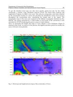
Another shortcoming of structured grids is their inability of accommodating a single block
to a complex geometry such as the one associated with the unstructured surface grid shown

in Fig. 2. Here, the geometry corresponds to that of the core shroud (moderator tank), with
cover, of a Boiling Water Reactor (BWR). The three-leg pillars that hold the cylindrical drum
of the steamdryer support (upper right corner of the view) may be observed at the edge of
the cover. In the forefront, the piping of the core spray system and a feedwater sparger has
been included in the figure. Steam separators that should have been connected to the outer
side of the core shroud cover, have not been displayed in the view of Fig. 2 in order to avoid
a forest of cylindrical shaped equipment that would have overloaded the view, rendering it
thickly. Only the trace of the connecting circular holes is seen in the core shroud cover.
A strategy to overcome the limitations of a single block structured grid consists of dividing
the computational domain in an appropriate number of regions, each one suitable for a
single block, i.e. to increase the number of structured grids, one for each block. But now, the
difficulties are moved to the issue of connecting the different blocks to build the complete
domain. Several block connection methods are available: the point-to-point method, in
which the blocks must match topologically and physically at the common boundary, the
many-to-one-point method, in which the blocks must match physically at the common
boundary, but be only topologically similar, and arbitrary connections, in which the blocks
must match physically at the common boundary, but may have significant topological
differences. Although the multi-block approach may increase the possibilities of achieving a
higher geometrical fidelity of the simulated flow system, the block connection requirements
may restrict the quality of the grids, which still are difficult to construct. Also, the price paid
by increasing the degrees of freedom in block connectivity is a detriment to the accuracy of
the solution and a deterioration in the solver robustness.
2.2 Unstructured grids, histogramming and polyhedra
In contrast to the limited possibilities of structured grids, Fig. 2 below constitutes a modest
indication of how far it might be possible to get with the requirement of geometrical fidelity
if an unstructured grid is used to fit a complex geometry. Unstructured grids lack the
mapping of the structured grids and, therefore, the information about the connection of each
node between physical space and computational space is kept within the algorithm of the
unstructured solver, which has to work out the location of the neighbours of each node, i.e.
the node at location “n” in memory may have no physical relation to the node next to it in

memory, at location “n+1”.
The disadvantages of unstructured grids are the need of larger computer resources and the
use of more complex algorithms that may not be as effective as those used with structured
grids under similar simulating conditions. Besides the aforementioned degree of
geometrical fidelity, unstructured grids have the great advantages of being easily
automatized in their generation, requiring limited time and effort in this process, and of
readily being suitable for spatial refinement. Depending on the grid generator, a minor
drawback with automatization might be the lack of user control when setting up the grid,
since most of the user participation may be restricted to disposing the mesh at the boundary
surfaces while the interior is automatically filled up by the software. Triangular and
tetrahedral elements are not easily deformed, i.e. stretched or twisted, leading to a grid that
may be rather isotropic, with elements of roughly the same size and shape. Rather than a
Numerical Simulation of Industrial Flows

235
disadvantage, this property may turn out to be of assistance for maintaining almost
everywhere in the computational domain a maximum element size of the grid that
adequately matches the size of the time step needed for resolving the different structures of
the flow to be simulated. Today’s possibility of treating the time dependence of the flow
with realistic accuracy is undoubtedly having an impact on the perception of grid quality,
an subject that will be further discussed in this work.


Fig. 2. Unstructured grid of the core shroud and cover of a BWR.
The traditional method for assessing grid quality, giving a statistical measure over the entire
computational domain, consists in histogramming (Woodard et al., 1992). Several
geometrical parameters are used to evaluate the quality of the individual elements, herein
assumed, without losing generality, to be tetrahedra since similar parameter definitions may
be obtained for any polyhedron. A few of such parameters are the minimum dihedral angle,
the ratio between the areas of the largest and the smallest faces and the volume ratio

between the smallest containing sphere and the largest contained sphere of the tetrahedron.
The minimum dihedral angle, which is the angle between two planes, is determined by the
scalar product of the combination of the four unity normal vectors corresponding to the
faces of the tetrahedron. The ratio between areas is found by the combination of the normal
vectors to each face obtained through the vector product of two of the three edges making
up a face. Although the information provided by these two indicators about the shape of
each element is similar, the evaluation of this area ratio is computationally far less
demanding than determining the dihedral angles for each face. The aforementioned volume
ratio is usually normalized by the value corresponding to a regular tetrahedron, which is
Numerical Simulations - Examples and Applications in Computational Fluid Dynamics

236
equal to 27 since the ratio of the radii of the spheres is 3. The ratio of the sphere radii, or its
inverse value, is generally used as aspect ratios.
Another important parameter for evaluating element quality is skewness, being it a measure
of the distortion of the element with respect to an ideal, equilateral element (i.e. regular
tetrahedron, cube, etc.). A method to estimate skewness, only valid for tetrahedra, consists
of the volume difference between the regular tetrahedron and the actual element shearing
the same circumsphere, normalized by the volume of the regular tetrahedron. A more
general method for skewness evaluation is the equiangle skew parameter defined by

⎥
⎦
⎤
⎢
⎣
⎡
−
−°
−

=
e
e
e
e
EAS
Q
θ
θθ
θ
θθ
minmax
,
180
max , (1)
where
θ
max
is the largest angle in face or cell,
θ
min
the smallest angle in face or cell and
θ
e
the
angle for equiangular face or cell, equal to 60° for tetrahedral and to 90° for hexahedral
elements (see e.g. Fluent, 2006). With the above definition, the equiangle skew parameter
will range between null and unity, being the maximum skewness value for an acceptable
grid not larger than 0.9.
Not only single element quality but also local grid quality needs to be quantified in order to

avoid large stretching and/or distorting of the grid. For instance, a doubling in the linear
spacing will result in an eightfold increase in volume, leading to large changes in volume
ratios. Even if these changes can be detected through analysis of the aforementioned volume
parameter, and the grid rectified, the flow structures to be resolved need an even
distribution of elements to maintain the accuracy of the simulation, as has already been
mentioned. Therefore, a limit in the grid spacing of the order of 10 %, rather than the one
normally accepted of about 20 %, should resolve this issue. The grid distortion can be
estimated by means of a skewness parameter defined by the ratio between the area of a
triangle formed with the center and the two nodes on each side of a chosen face, and the
area of the face. If two elements are perfectly aligned, the area of the formed triangle is zero,
indicating a local nonexistence of grid skewness.
Grid diagnosis using a methodology of the kind discussed above leads to the necessity of
modifying the grid based not only on geometrical criteria but also on concrete physical
criteria in order to objectively improve the quality of the grid to be used for the specific flow
simulation. As was expressed at the beginning of this section, the grid reflects the simulation
problem to be solved and should, consequently, be individual in its quality to conform to
the associated physical problem. Therefore, the first, a priori, constructed grid following the
aforementioned guidelines will seldom be optimal for the assigned task and will need to be
customized through an iterative procedure to comply with the conditions of the physics
involved in the simulation. A typical example of this situation is the need for grid
refinement in order to capture shocks in aerodynamic applications (see e. g. Borouchaki &
Frey, 1998, Acikgoz, 2007). The adaptation is normally achieved using the pressure gradient
of the solution as an indicator and, in all probability, the adaptation procedure needs to be
repeated several times in order to attain an optimal solution of the grid valid for the specific
application.
A particular issue related to grid refinement, which needs special attention due to the
connections to other physical phenomena like turbulence and heat transfer, is that of the
near wall regions of the flow where large velocity gradients are present, i.e. the boundary
layers. In turbulent flows, the wall region is dominated by the effect of shear stress and very
Numerical Simulation of Industrial Flows

237
close to the wall, at the viscous sublayer, the scaling parameters are the kinematic viscosity
of the fluid and the shear stress at the wall. The characteristic velocity and length scales
there are the friction velocity, the square root of the quotient of the shear stress at the wall
and the fluid density, and the viscous length scale, the quotient of the kinematic viscosity of
the fluid and the friction velocity. Based on these scales, the non-dimensional normal
distance to the wall may be expressed in wall units as

ν
τ
yu
y =
+
, (2)
where y is the dimensional normal distance to the wall, u
τ
the friction velocity and
ν
the
kinematic viscosity of the fluid. This distance in wall units is a dynamic measure of the
relative importance of viscous and turbulence transport within the boundary layer that
affects wall friction, heat transfer, buoyancy and other related physical phenomena.
Depending on the degree of approximation of the simulation, a certain minimum value of y
+

is required for the resolution of the computational cells adjacent to the wall in order to
capture the correct wall phenomena to the desired level of accuracy.
Further considerations to be presented in the next sections establish that it is turbulence
modeling that primarily defines the near wall grid resolution. Additional requirements not

only on the normal distance to wall, may however arise due to, for instance, conjugate heat
transfer (CHT), natural convection, etc. In the end, the near-wall resolution of the grid is, as
the rest of it, solution dependent and has to be optimized by means of refinement through
an iterative process.
Finally, some words should be added about the future of grid development. Tetrahedral
grids have several already mentioned advantages, but need much larger number of
elements for a given volume than grids using other geometrical elements as, for instance,
hexahedra, resulting in higher requirements in memory storage and computing time. A
tetrahedral control volume has only four neighbors, a property that may deteriorate the
computation of gradients in all needed directions. If the neighbor nodes are inadequately
located, for example all lying nearly in the same plane, the evaluated gradient normal to that
plane may be marred by a large uncertainty. A solution to this and other problems with
tetrahedral grids is the use of elements of more complex geometrical shape, i.e. polyhedra
(see e.g. Peric, 2004). According to this reference, about four times fewer cells, half the
memory and a tenth to a fifth of computing time are needed with polyhedral grids
compared to tetrahedral grids for achieving the same level of accuracy of the solution. Two
alternatives are now available for generating polyhedral grids, the first to generate the
polyhedral grid from scratch and the second to convert tetrahedra to polyhedra from an
already existing grid. The later possibility has been tested by the authors with clearly
approved result that will be further commented in the next sections (see e.g. Figures 8
and 9).
As will be explained later on, a minimum spatial size of the grid is necessary for a required
level of resolution of the turbulent, time dependent structures of the flow, and the feature of
polyhedral grids of containing fewer, larger cells may not necessarily be a clear advantage in
this kind of simulations. As in every new area of development, more quantitative
examination of the properties of polyhedral grids, especially in turbulent, time dependent
applications, is needed to get a complete understanding of the virtues of polyhedral
elements in industrial simulations.