Đo nhiệt độ P1 pdf
Bạn đang xem bản rút gọn của tài liệu. Xem và tải ngay bản đầy đủ của tài liệu tại đây (1.13 MB, 18 trang )
1
Temperature
Scales
and
Classification
of
Thermometers
1
.1
Temperature
-
Historical
Background
The
concept
of
temperature
makes
one
think
of
physiological
experiences
whilst
touching
or
approaching
some
solid
.
Some
of them
may
be
described
as
cold,
cool
or
tepid,
others as
hot
or
warm
.
Warmer
bodies
transfer
heat
to other
cooler
bodies
.
Both
bodies
tend
to
equalise
their
temperatures,
approaching
a
new
common
intermediate
temperature
.
Thus
the
correctness
of
the
definition,
given
to
temperature
by
the
Scotsman
James
Clerk
Maxwell,
may
be
seen
.
He
stated
that
the
temperature
ofa
body
is its
thermal
state,
regarded
as a
measure
of
its
ability
to
transfer
heat
to
other
bodies
.
At
the
present
time,
this
definition
compels
the
attribution
of
larger
numerical
values
to
those
bodies
which
have
a
higher
ability
to
transfer
heat
to
other
bodies
.
This
definition
forms
the
basis
of
all
of
the
international
temperature
scales
in
use
both
presently
and
in
the
past
.
Science
took
a long,
difficult
and
tortuous
route,
full
of
errors,
to this
contemporary
definition
of
temperature
.
In
ancient
Rome,
during
the
second
century
BC,
the
physician
C
.
Galen
introduced
four
degrees
of
coldness
regarding
the
effects
of
different
medicines
upon
human
organisms
.
These
medicines
were
supposed
either
to
warm
or
to
cool
them
.
Galen
also
introduced
a
neutral
temperature,
attributing
to
it
a
value
of
zero
degrees
.
He
claimed
that
this
neutral
temperature
depended
upon
geographical
latitude
.
The
first
device,
which
was
used
to
measure
the
degree
of
warmth
or
coldness,
seems
to
have
been
invented
by
Galileo
Galilei
some
time
between
the
years
1592
and
1603
.
This
instrument,
which
is
shown
in
Figure
1 .1,
consisted
of
a glass
bulb
connected
to
a
long
tube
immersed
in
a
coloured
liquid
.
After
a
preliminary
heating
of
the
contained
gas,
its
subsequent
cooling
caused
a
certain
amount
of
the
liquid
to
be sucked
in
.
The
liquid
column
rose
or
fell
as a
function
of
the
ambient
temperature
.
In
the
absence
of
any
evidence
that
the
instrument
had any
graduation,
it
is
better
to call
it
a
thermoscope
.
As
the indicated
values
were
also
a
function
of
the
atmospheric
pressure
its
precision
must
have
been
quite
poor
.
Subsequently,
about
the
year
1650,
the
members
of
the
Florentine
Academy
of
Sciences
made
the
first
thermometer,
which
is
represented
in
Figure
1
.2
.
This
consisted
of
a
spiral
shaped
tube
with
a
closed
end and
a
graduation
.
However,
no
numbers
were
ascribed
to the
graduation
marks
(Lindsay,
1962)
.
In
the
course
of
time
the
need
arose
to
define
temperature
fixed
points,
to
standardise
those
thermometers
which
existed
at
that
time
.
One
of
the
first
proposals
came,
in 1669,
Temperature Measurement Second Edition
L. Michalski, K. Eckersdorf, J. Kucharski, J. McGhee
Copyright © 2001 John Wiley & Sons Ltd
ISBNs: 0-471-86779-9 (Hardback); 0-470-84613-5 (Electronic)
2
TEMPERATURE
SCALES
AND
CLASSIFICATION
OF
THERMOMETERS
Figure
1
.1
Galileo's
air
thermoscope
(1592)
Figure
1 .2
Thermometer
of
the
Florentine
Academy
of
Sciences
(1650)
from
H
.
Fabri
from
Leida
.
His
proposal
was
for
two
fixed points
.
The
lower
should
be
the
temperature
of
snow
and
the
higher
the
temperature
of
the
hottest
summer
day
.
A
later
proposal,
which
was
made
by
C
.
Rinaldi
from
Padua
in
1693,
suggested
that
the
fixed
points
should be
the
temperatures
corresponding
to
the
melting
point
of
ice
and
the
boiling
point
of
water
.
Between
these
two
points,
twelve
divisions
should
be
introduced
.
In
the
same
year,
and
for
the
first
time,
the
British
scientist
E
.
Halley
applied
mercury
as a
thermometric
liquid
.
Remer,
a
thermometrist
working
in
Copenhagen
at
the
end
of
the
17th
and
beginning
of
the
18th
century,
developed
a scale
where
zero degrees
was
associated
with
the coldest day,
while
the
normal
temperature
of
the
human
body was
associated with
24°
.
This
made
the
temperature
of
boiling
water
equivalent
to
gt
50
°
-55
°
on
this
unusual
scale,
which
was
influenced
by
the
predominant
use
of thermometers
for
meteorological
purposes
at
that
time
.
Hence,
if
the
freezing
point
of
water
had
been
taken
as
zero,
the
repeated
use
of
negative
values
for
winter
temperatures
would
have
occurred
.
Winter
temperatures
of
-16
°
C
(
;
z~
0
°
F) are quite
common
in continental
Europe
.
A
further
notable
milestone
in
thermometry
is
due
to
D
.
G
.
Fahrenheit
from
Danzig
(now
the
city
of
Gdansk
in
Poland),
who
visited
Romer's
laboratory
shortly
after
Romer
proposed
his
scale
.
To
avoid
the
problems
associated
with
Romer's
scale,
it
seemed
obvious
to
Fahrenheit
to
use
the
lowest
attainable
temperature
of
those
days
as
zero
.
As
a
result,
Fahrenheit
developed
the
specification
and
use
of
the
mercury-in-glass
thermometer
in
1724
.
Evidently
influenced
by
Romer's
scale,
he
proposed
his
own,
very
well
known
scale
.
This
scale,
called
the
Fahrenheit
scale,
which
persists
today,
is
essentially
the
same
as
that
described
by him
to
The
Royal
Society
in
1724
.
Fahrenheit
described
the
mercury-in-glass
thermometer,
introducing
three
temperature
fixed
points
:
THERMODYNAMIC
TEMPERATURE
SCALE
(TTS)
3
"
A
mixture
of
ice,
water
and
ammonium
chloride
was
taken
as the zero point
.
"
A
mixture
of
ice
and
water
was
taken
as
32°
.
"
A
human
body
temperature
was
taken
as
96°
.
Even
yet there
is
no
clear
reason
why
Fahrenheit
chose
such
a scale division
based
upon
these
assumed
temperature
fixed points
.
As
Newton
Friend (1937)
indicated,
the
reasons
for
choosing such
a scale division
by
Fahrenheit
might
have
been
that
in
the eighteenth
century
the
majority
of
thermometers
were
intended
for
meteorological
purposes
.
Taking
the
freezing point
of
water
as
zero
would
have
involved
the
repeated
use
of
negative
values
for
winter
temperatures
.
To
avoid
this,
Fahrenheit
proposed
to
use
the
lowest
attainable
temperature
of
those
days
as zero
.
In the
case
of
the
upper
fixed
point,
the
temperature
of
boiling
water
was
rejected
as
being
unnecessarily
high
for
meteorological
purposes
.
In
his
decision
to
assume
96°
for the
temperature
of
the
body,
Fahrenheit
was
influenced
by
the
already
existing
Remer
scale
.
He
merely
changed
Romer's
24
degrees
for
body
temperature
to
96
.
This change,
which
was
equivalent
to
four
subdivisions
on
each
degree
;
of
the
Romer
scale,
was
also
probably
made
because
96
is
divisible
not
only
by 2
but
also
by
multiples
of
3
and
hence
12
.
The
decimal
system
was
not
in general
use
at that
time
.
Further
development
of
the
mercury-in-glass
thermometer,
in
1742,
was due
to
the
Swedish
astronomer
and
physicist
A
.
Celsius
.
He
assigned
0° to
the
temperature
of
boiling
water
and
100°
to the
temperature
of
melting
ice
.
The
region
between
these
two
points
was
divided
into
100
equal
steps
.
Subsequently,
after
the
death
of
Celsius
in
1744,
M
.
Stromer,
friend
and
scientific
collaborator
of
Celsius,
reversed
these
values
.
Eventually, as
science
developed,
a
need
to
measure
temperatures
above
the
melting
point
of
glass arose
.
Prinsep's
air
thermometer,
which
used
a
gold bulb
to
measure
temperatures
of
1000
0
C
in
1828,
was
followed
soon
after,
in
1836,
by
a
platinum
bulb
in
a
similar
thermometer
by
Pouillet
.
A
true
Thermodynamic
Temperature
Scale
(TTS),
described
below,
had
been
the
unconscious
aim
of
all
of
the
previous
efforts
.
Such
a
scale
was
not
possible
until
1854
when
its
foundations
were
laid
by
the Belfast
born
William
Thomson,
who
later
became
Professor
of
Natural
Philosophy
in the
University
of
Glasgow,
Scotland,
and
assumed
the
title
Lord
Kelvin of
Largs
.
Of
course, the
aim
of
any
scale
of
temperature,
but
especially
the
thermodynamic
scale,
is
the representation
of
the
hotness
relations
between
objects
and
events
in
the
real
physical
world
by
numbers
.
1
.2
Thermodynamic
Temperature
Scale
(TTS)
The aim
of
any
scale
of
temperature,
but especially the
thermodynamic
scale,
is
the
representation
of
hotness
and
hotness
relations
between
objects
and
events
in
the
real
physical
world
by
real
numbers
.
As
numerical
values are correlated
to
some
defined
temperatures,
temperature
faxed
points
are
required
to
characteristic
certain
values
of
temperature
.
Interpolation
then
allows
the
definition
of
temperature
between
these
temperature
fixed
points
.
To
enable
some
defined
interpolation
between
these
temperature
fixed
points,
a
thermometric
working
substance,
one
of
its
properties
and
a correlating
function
must
be
assumed
.
The
chosen
function
provides
the
means
of
associating the
specific
property
of
the
working
substance
with
a
certain
temperature
.
Because
of
the
diversity
of
materials
and
4
TEMPERATURE
SCALES
AND
CLASSIFICATION
OF
THERMOMETERS
their
properties there
is
an
unlimited
number
of
these
temperature
scales
.
Properties
which
may
be
relevant
are,
for
example,
the
length
of
a
rod,
the
pressure
of
saturated
steam,
the
resistance
of
a
wire
and
so
on
.
In
the
given
temperature
range
the
property
must
be
consistently
repeatable
and
reproducible
.
In
normal
conditions,
corresponding
to
101
.325 kPa,
let
the
ice-point
temperature
be
0°
and
the
temperature
of
boiling
water
be
100°
.
Assuming
that
the
chosen
property
is
linearly
dependent
upon
the
temperature
it
is
apparent
that
any
temperature
scale
based
upon
say
the
thermal
expansion
of
a
copper
rod,
will
not
coincide
with
a
scale
based
upon
the
thermal
expansion
of
another
metal
or on
any
changeof
its
resistance
with temperature
.
The
material,
which
most
closely
approximates
this
ideal
thermometric
working
substance,
is
an
ideal
gas
.
Indeed
it
was
the
work
of
Robert
Boyle
and
his
co-workers
in
the
middle
of
the
17th
century
which
led to
the
conviction
of
many
later
scientists
that
there
was
such
a thing
as
an
absolute zero
of
temperature
.
These
eminent
individuals
included
G
.
Amontons,
in
Paris
in
1699,
J
.
H
.
Lambert,
in
1770,
and
Gay-Lussac,
in
1790
.
Gay-Lussac
gave
credit
to
J
.
A
.
C
.
Charles
for
that
individual's
previously
unpublished
research
.
All
of
their
efforts
resulted
in
what
is
now
called
the ideal
gas
law,
also
called
the
Boyle-Mariotte
law
which
is
written
in
the usual
form
:
pV
==
nkT
(1
.1)
where
p
is
the
pressure,
V
is
the
volume,
n
is
the
number
of
moles
of
gas,
k=
1
.3807
x
10
-23
J/K
is
Boltzman's
constant
and
T
is
the
absolute
temperature
.
When
the
temperature
is
held
constant,
equation
(1
.1)
corresponds
to
Boyle's
law
.
Similarly
Charles'
law
is
obtained
from
equation
(1
.1)
when
the
pressure
is
held
constant
.
Since
there
are
no
direct
methods
for
measuring
temperature,
as there
are
with
say
length
measurement,
difficulties
are
associated
with
temperature
measurement
.
As
only
associative
temperature
measurements
are
possible,
any
temperature
scale
depends
upon
the
chosen
thermometric
working
substance
and
its
chosen
property
.
Although
any
working
substance
may
be
employed
in
principle,
it
will
be
restricted
to
some
finite
range determined
by
its
thermal
behaviour
.
For
example,
the
application
of
mercury-in-glass
thermometers
is
limited
on
the
low-temperature
side
by
the
solidification
of
the
mercury
as
it
freezes
and
on
the
high-temperature
side
by
the
inability
of
the
glass
to
expand
indefinitely
as well as
its
melting
temperature
.
Melting
of
the
glass
was
responsible
for
the
development
of
the
Prinsep
and
Pouillet
thermometers
.
An
ideal
solution
to the
problem
of
proposing
a
suitable
temperature
scale
would
be
to
find
one
valid
in
any
temperature
range
and
totally
independent
of
the
working
substance
.
The
thermodynamic
Kelvin
Scale,
based
upon
the
efficiency
of
the
ideal
reversible
Carnot
cycle,
is
such
a
scale
(Herzfeld,
1962
;
McGee,
1988)
.
A
reversible
Carnot
cycle,
which
is
impossible
to
realise
in
practice,
consists
of
a
.
reversible
heat
engine
operating
between
two
isotherms
at
the
temperatures
T2
and
T
I ,
with
T
2
>
T
I
,
and
of
two
adiabatic
processes
.
A
reversible
heat
engine
absorbs
the
heat,
Q
2
,
from
the
high-temperature
source,
at
the
temperature
T
2
,
and
discharges
the
heat
Q
t
to
the
low-temperature
source,
at
the
temperature
Ti
.
The
difference
between
the
absorbed
heat
Q2
and
the
discharged
heat
Q
t
,
which
is
the
external
work,
A,
performed
by
the
engine,
may
be
written
as
:
A
=Q2
-
Qt
(1 .2)
THERMODYNAMIC
TEMPERATURE
SCALE
(TTS)
5
Reversing
the
engine
action,
indicates
that
it
may
be
driven
by
a
second
identical
engine,
workingbetween
the
same
two
heat
sources
.
The
effect
of such
action
might
be
the heat
flow
from
the
lower
to the
higher
temperature
;
source
.
Using
the
properties
of
reversible
processes
it
may
be
proven
that
the
ratio
Q2
./Q1
is
a
function
only
of
the
two
source
temperatures,
so
that
:
Ql
_f(T2,Ti)
(1
.3)
Following
Kelvin's
proposal
it
may
be
assumed
.
that
the functional
relation
in
equation(L3)
is
:
Q2
-
T2
(1
.4)
Q1
Ti
Equation
(1
.3)
is
the
basis
of
the
TTS
and
thus the efficiency
of
a
reversible
heat
engine
is
defined
as
:
Q2
T2 T2
This
efficiency
and
the
definition
of
temperature,
which
is
based
upon
it,
may
be
shown
to
be
independent
of
the
working
substance
.
As
a
result
it
may
be used
to
define
the
TTS
:
T
=T2(1-t1)
(1
.6)
By
means
of
this
scale
any chosen
thermal
state
such
as the
melting
point
of
ice,
may
be
assigned
a
certain
value
of
thermodynamic
temperature
.
The
TTSmay
be
founded
upon
a
defined
temperature
difference
between
two
temperature
fixed points
or
on
a
defined
value
of
one
temperature
fixed point
.
In the
course
of
the
development
of
technology,
the
manner
of
defining
the
TTS
has
changed
.
Until
1954,
it
was
assumed
that
100°
represented
the difference
between
the
boiling
point
of
water
and
the
melting
point
of
ice
.
Since
then,
there
has
been
a
return
to
the
original
and
older proposals
of
Kelvin,
in
1848,
Mendeleyev,
in
1874,
and
Giauque
in
1939
.
Thus,
since
1954,
the
TTS
is
based
upon
one
temperature
fixed
point,
which
is
the
triple
point
of
water
.
Triple points
of
physical
materials
are
stable,
repeatable
temperatures
where
the
solid,
liquid
and
gaseous
forms
of
the material
exist
in
thermal
equilibrium
.
The
triple
point
of
water
occurs
at that
temperature
when,
ice,
water
and
water
vapour
exist
in
thermal
equilibrium
.
A
temperature
of
273
.16
has
been
assigned
to this
temperature
fixed
point
.
In
1967
the
Thirteenth
General
Conference
on
Weights
and
Measures
(CGPM)
introduced
a
new
definition
for the
scale
and
a
new
symbol
for the
unit
of
thermodynamic
temperature
.
This
unit
is
called
the
kelvin
denoted
by
the
symbol
K
.
In the
S1,
when
units
are
called
after
people,
the
unit
name
always
starts
with
a
small
letter to
emphasise
that
it
is
the
unit
being
referred
to,
not
the
person
.
It
is
defined
as
1/273
.16
part
of
the
thermodynamic
temperature
of
the
triple
point
of
water
.
6
TEMPERATURE
SCALES
AND
CLASSIFICATION
OF
THERMOMETERS
Even
though
the
Carnot
cycle
cannot
be
realised
in
practice,
it
can
be
demonstrated
using
equation
(1
.1)
that
the
thermodynamic
scale
may
be reproduced
by
a
gas
thermometer
with
an
ideal
gas as the
working
substance
.
Here
again,
although
the
ideal
gas
is
quite
fictitious,
it
could
be
replaced
by
a
noble
gas
at
very
low
pressure
.
Either
pressure
difference
at
constant
volume
or
volume
difference
at
constant
pressure
can
be chosen
as
the
measure
of
temperature
.
When
the
readings
of
temperature
at
constant
volume,
T
,
and
the similar
readings
at
constant
pressure,
T
p
,
are
extrapolated
to
zero they
tend
to
the
same
value
T
= T
p
=
T,
independently
of
the
properties
of
the
gas
.
Thus,
the
TTS
may
be
reproduced
using
gas
thermometers
which
have
an
application
range
up
to
about
1350
K
.
Another
simple
methodof
reproducing
the
scale
at
thermodynamic
temperatures
above
1337
K
is
allowed
bymeans
of
thermal
radiation
from
heatedbodies
.
When
this
radiation
is
in
thermodynamic
equilibrium
with
the
radiating
body,
some
properties
of
this
radiation
are
directly
linked
to
the
temperature
of
the
body
(Herzfeld,
1962)
.
The
concepts
of
black
body
radiation are
essential
for
proper
utilisation
of
the
method
.
For
thermal
radiation
to
possess
similar properties
to
that
from
black
body
radiators
it
should
be
emitted
from
an
aperture
which
is
sufficiently
deep
and narrow
with
a
uniform
temperature
distribution
in
accordance
with
the
principles
given
in
Section
8
.2
.
When
these
conditions
are
complied
with,
it
may
be
shown
that
the
radiation
intensity
and
its
spectral
distribution
only
depend
upon
the
temperature
of
the
body
and
not
upon
its
material
.
Take,
as a reference
system,
a
heated
body,
which
is
radiating
heat with
some
radiation
intensity
and
whose
temperature,
T
,
is
within
the
measurement
range
of
a gas
thermometer
.
The
radiant
intensity
of
the
body
provides
a
means
of
extending
the
TTS
to
higher
temperatures
.
A
relation
between
the
ratio
of
spectral
radiant
intensities
of
a
black
body
at
two
different
temperatures,
T and
T
2
,
at
one
wavelength,
A,
exists
.
This
relation
is
obtained
from
Planck's
law
(given
later
in
equation
(8
.7))
which
is
:
W
;LT
e
c2/
,
I T,
_
1
`
c
lRT
(1
.7)
WA
T2
e
2
t_1
where
WA
T
and
WX
T
are
the
spectral
radiant
intensities
of
a
black
body
at
the
temperatures
T
and
T
2
respectively,
c2
=
0
.014
388
m
K
is
Planck's
constant,
and
i1
is
the
wavelength
in
metres
.
Equation
(1
.7)
presents the
ratio
of
the
spectral
radiant
intensities
of
a
black
body
at
two
temperatures
T
i
and
T
2
at
the
same
single
wavelength,
A,
.
The
temperature
T
2
is
to
be
determined,
whereas
T
is
the
temperature
of
a fixed
point
measured
by
a gas
thermometer
.
1
.3
International
Temperature
Scales
1
.3
.1
From
the
Normal
Hydrogen
Scale
to
EPT-76
A
primary
standard
system
for
measuring
temperature
is
the
"Kelvin
Thermodynamic
Temperature
Scale"
referred
to
above
.
Because
of
the
difficulties
which
are
involved
in
INTERNATIONAL
TEMPERATURE
SCALES
7
realising
this
primary
standard system,
widely
accepted
realisations
are
based
upon
boiling
points,
freezing/melting
points
and
triple
points
.
Boiling
points
correspond
to
characteristic
temperatures
where
the
liquid
and
gaseous
states
of
a material
exist
in
equilibrium
.
Freezing/melting points
are
temperatures
where
a material
undergoes
an
equilibrium
change
in
its
physical
state
from
liquid
to
solid
or
solid
to
liquid
respectively
.
Freezing/melting
points
are
preferred
to
boiling
points
as
they
are
less sensitive
to
pressure
changes
.
Triple
points
are
temperatures
where
the
solid liquid
and
gaseous forms
of
the
material
exist
in
equilibrium
.
Practical
realisations
of
temperature
scales
have
been
disseminated
by
previously
adopted
resolutions
of
the
CGPM
in
1889, 1927,
1948
(revised
in
1960),
1968
(supplemented
in
1976)
and
1990
.
For
comparative
purposes
all
of
these
scales
are
summarised
in
Figure
1
.3
.
The Normal
Hydrogen
Scale,
or
NHS,
which
was
based
upon
the
work
conducted
by
Chappuis
(1888),
a
staff
member
of
the
International
Bureau
of
Weights
and
Measures
(BIPM),
was
proposed
by
the
International
Committee
of
Weights
and
Measures
(CIPM)
in
1887
.
Using
hydrogen
gas
as the
thermometric
material,
Chappuis
built
a
gas
thermometer
GAS
THERMOMETER
-
-25
C
100
°C
-
PLATINUM
RESISTANCE
90%Pt-10%Rh
I
Pt
RADIATION
THERMOMETER
THERMOCOUPLE
THERMOMETER
-198
'C
(2
Sub-ranges)
660
C
1063
C
PLATINUM
RESISTANCE
THERMOMETER
90%Pt-10%Rh
l
Pt
RADIATION
(2
Sub-ranges)
(THERMOCOUPLE
THERMOMETER
183
°C
660
C~
. .
1063
C
'`
PLATINUM
RESISTANCE
90%Pt-10%Rh
l
Pt
RADIATION
THERMOMETER
THERMOCOUPLE,
THERMOMETER
13
.
(2
Sub-ranges)
I
~
81
K
6
30
.74 'C
^-064.43
W
PLATINUM
RESISTANCE
RADIATION
THERMOMETER
(3
Structures
cover
11
Sub-ranges)
`
:'
THERMOMETER
13
.8_0_3
K
961
.78
VAPOUR
~t
GAS
PRESSURE
THERMOMETER
(0
.65
K
to
5
K)(3
K
to
24
.5561
K
0
500
1000
TEMPERATURE,
°C
Figure
1 .3
Comparison
of
the
various
temperature
measurement
scales
and
the
measuring
ranges
of
their
standard
interpolating
instruments
or
sensors
8
TEMPERATURE
SCALES
AND
CLASSIFICATION
OF
THERMOMETERS
calibration
facility
covering
the
range
-25
°
C
to
+100
°
C
.
This
early
scale,
which
was
used
to
calibrate
mercury-in-glass
thermometers,
was
a
true
centigrade
scale
as
its
fixed points
were
the
ice-point,
at
0
°
C,
and
the
boiling
point
of
water,
at
100
°
C
.
A
gas
thermometer
is
a
complex
piece
of
apparatus
which
is
only
appropriate
for
use
as
a
primary
standard
in
fundamental
laboratory
measurements
.
Since
this
severely
limits
its
practical use,
the
gas
thermometer
needs
to
be
replaced
by some
other,
more
practically
convenient
types
.
To
this
aim,
in
1911,
Germany,
Great
Britain
and
USA
agreed
to
accept
one
common,
practical
temperature
scale,
but
its
completion
was
delayed
by
the
outbreak
of
World
War
1
.
When
it
was
defined
in
1927
by
the
Seventh
General
Conference
on
Weights
and
Measures
with
the
assignment
of
six
defining
or
fixed
points,
it
was
called
the
International
Temperature
Scale
of 1927
(ITS-27)
.
Development
of
thermometers
using
the
noble metal
platinum,
giving
rise to
the
Platinum
Resistance
Thermometer,
or
PRT,
followed
the
pioneering
groundwork
of
Siemens,
in
1871,
and
Callendar, in
1887
.
By
the
end
of
World
War
I,
PRTs
were
acknowledged
as
precision
thermometers
.
This
confidence
provided
the basis for
their
specification
as
one
of
the
standard
interpolating
instruments
of
ITS-27
.
Over
the
range
-190
°
C
to
+
660
°
C, in the
sub-ranges
-190
°
C
to 0
°
C
and
0
°
C
to
660
°
C,
the
interpolating
instrument
was
specified
as the
PRT
made
from
platinum
with
defined
properties,
exhibiting
resistances
at
three
temperatures,
expressed
as
ratios
with
respect
to the
resistance
at
0
°
C
.
From
660
°
C
to
1063
°
C
the scale
was
to
be
interpolated
using
a
platinum-10%
rhodium
/platinum
(90%Pt-10%Rh/Pt)
thermocouple
made
from
materials
with
specified
properties
.
The
Wien's
law
defined
temperatures
above
1063
°
C
.
ITS-27
was
a
major
step
forward
in
the
universality
of thermometry
as
it
removed
previously
observed
ambiguities
in the
specification
of
temperature
.
The
tortuous
path
in
the
development
of
a
temperature
scale,
which
truly
represented
the
thermodynamic
scale,
soon
uncovered
the
inadequacies
of
ITS-27
.
Thus was
born
the
International
Temperature
Scale
of 1948
(ITS-48),
which
possessed
the
same number
of
fixed points as
ITS-27,
but
with
the freezing
point
of
silver
now
specified
as
960
.9'C,
instead
of
960
.5 °
C
as
in
ITS-27
.
The
lower
PRT
interpolating
limit
was
also
raised
to
-183
°
C
to
coincide
with
the
oxygen
boiling
point
of -182
.970'C
.
Otherwise
the
PRT
standard
interpolation
sub-ranges
remained
the
same,
as
well
as
that
of
the
90%Pt-10%Rh/Pt
interpolating
thermocouple
.
In the
case
of
the
interpolating
thermocouple,
a
quadratic
interpolating
equation
was
introduced
with
new
constraints
placed
upon
the
acceptable
values
and
tolerances
of
the
em£
Above
1063
°
C,
Wien's
law
was
replaced
by
Planck's
law
to
improve
the
thermodynamic
consistency
of
the
temperatures
in this
range
and
also
to
allow
the
use
of
ITS-48
at
higher
temperatures than
ITS-27
.
In
1960,
a revision
of ITS-48
became
known
as
the
International
Practical
Temperature
Scale
of
1948(60),
or
IPTS-48(60),
to
avoid
confusion
with
ITS-48
.
The
changes,
which
specified
the
water
triple
point
temperature
as
273
.16
K,
creating
the
present
Kelvin
Thermodynamic
Scale,
also
included
its
adoption
as a fixed point
of
the
scale
in
place
of
the
ice-point
temperature
.
The
name
of
the
unit
of
temperature
was
changed
to
degrees
Celsius,
°C,
in
place
of
centigrade
.
ITS-47
was
a
true
centigrade
scale
as
it
had
100
degrees
as
the
fundamental
interval
between
the
ice-point
and
the
water
boiling
point
.
As
the freezing point
of
zinc,
at
419
.505
°
C,
was more
precisely
realised,
it
was
proposed
as
a
replacement
for
the
sulphur
boiling
point
at
444
.60
°
C
.
New
restrictions
were
placed
upon
one
of
the
PRT
ratios
and
upon
the
standard
thermocouple
emf
.
The
International
Practical
Temperature
Scale
of
1968, or
IPTS-68,
which
was
based
upon
boiling points,
melting/f~eezing
points
and
triple
points,
arose
from
the
need
to
extend
INTERNATIONAL
TEMPERATURE
SCALES
9
IPTS-48
to
lower
temperatures
as
well
as
from improved
measurement
methods
.
A
total
of
thirteen
fixed
points
were
used
to
define
the
scale
.
Although
the
interpolating
instruments
were
the
same
as
for
IPTS-48,
the
PRT
range
was
extended
to
cover
the
lower
temperature
region
down
to 13
.8
K,
using
four
wire
resistance
connections
in
two
different
sensor
structures
.
The
scale
was
also
more
closely
defined
in
terms
of
a reference
function,
with
four
different
deviation
functions
defined
to
provide
correction
in
the
four
different
temperature
sub-ranges
for the
particular
PRT
being
calibrated
.
In the
original
statement
of
IPTS-68,
the
same
90%Pt-l0%Rh/Pt
thermocouple
covered
the
same
range
as
in
IPTS-
48(60)
with
the
same
quadratic
form
for
the
emf
defining
equation
.
The
range
of
application
of
this
thermocouple,
subsequently
adopted
by
the 15th
CGPM
in
1975,
was
changed
to
630,74
°
C
to
1064,43
°
C
in
IPTS-68(75)
with
a
commensurate
tightening
of
the
emf
specifications
.
Above
1064
.43
°
C,
Planck's
law
defined
the
scale
.
An
Extended
Practical
Temperature
Scale
of
1976,
or
EPT-76,
which
includes
revisions
to
IPTS-68,
allowed
IPTS-68
to
be
extended
at
low
temperatures with
the addition
of
11 fixed points
in
the
cryogenic
range
from
the
super-conducting
transition
point
of
cadmium
at
0
.519
K
to
the
boiling
point
of
neon
at
27
.102
K
.
1
.3 .2
The
International
Temperature
Scale
of
1990
(ITS-90)
IPTS-68
and
EPT-76
have
now
been
superseded
by
the
International
Temperature
Scale
of
1990,
also called
ITS-90
for
brevity,
which
was
adopted
by
the
International
Committee
of
Weights
and
Measures
in
September
1989
.
(NPL,
1989
;
Preston-Thomas,
1990
;
Rusby,
1987)
.
The
differences
existing
between
values
of
ITS-90 and
of
ITS-68
are
of
no
practical
influence
in
industrial
measurements
.
The
scale
is
established
by
correlating
some
temperature
values
with
a
number
of
well
reproducible
equilibrium
states
(i .e
.
the
temperature
fixed
points),
which
define
the
primary
standards
to
be
used
and
gives
the
interpolating
equations
for
calculating
temperatures
between
the fixed points
.
More
details
about
the
PRT
interpolating
equations
are
given
in
Chapter
4
.
Planck's
law
is
used
to
define
ITS-90
above
the freezing
point
of
silver
.
Overall,
ITS-90
represents
Thermodynamic
Temperature
with
an
uncertainty
of
±2
mK
from
1
K
to
273
K
increasing
to
±7
mK
at
900
K
.
The
unit
:
of
TTS
is
the kelvin,
symbol
K
.
One
kelvin
is
defined
as
1/273
.16
of
the
thermodynamic
temperature
of
the
triple
point
of
water
.
Celsius
temperature
is
expressed
as
:
t(
°
C)
=
T(K)
-
273
.15
(1
.8)
The
unit
of
Celsius
temperature
is
degree
Celsius,
symbol
°
C,
which
equals
one
kelvin
.
The
temperature
difference
is
expressed
either
in
kclvins
or
°
C
.
In
ITS-90
a
distinction
exists
between
the
International
Kelvin
Temperature,
T
90
,
and
the
International
Celsius
Temperature,
t
9o
,
where
t
9o (°
C)=T
9o
(K)
-
273
.15
(1
.9)
In
this
book
the
Celsius
temperature
will
be
indicated
by
23
to
avoid
confusion
with
the
unit
of
time,
which
is
indicated
by
t
.
10
TEMPERATURE
SCALES
AND
CLASSIFICATION
OF
THERMOMETERS
Interpolation
between
the
Defining
Fixed
points
of
ITS-90,
listed in
Table
1 .1,
are
as
follows
.
1
.
From
0
.65
K
to 5
.0
K
:
T
90
is
defined
in
terms
of
the
vapour
pressure
temperature
relations
of
3
He
and
4
He
.
2
.
From
3
.0
K
to
24
.5561
K
(the
triple
point
of
neon)
:
the
constant
volume
type
of
3
He
or
4
He
gas
thermometer
is
used
.
It
is
calibrated
at
three
experimentally
realisable
temperatures
of
defining fixed
points
using
specified
interpolation
procedures
.
3
.
From
13
.8033
K
(the
triple
point
of
equilibrium
hydrogen)
to
961
.78
°
C
(the
freezing
point
of
silver)
:
the
standard
instrument
is
a
platinum
resistance
thermometer
calibrated
at
specified
sets
of
defining
fixed points
and
using
specified
interpolation
procedures
.
As
indicated in
Figure
1 .3
and
described
by
Nicholas
and
White
(1994),
Pt
thermometers
with
3
different
structures
are
used
in
11
different
temperature
sub-ranges
.
The
temperatures
are
determinedfrom
the
reduced
thermometer
resistance
ratio,
defined
by
the
relation
:
W(T90)
=
R(T90)
(1
.10)
R(273
.16
K)
Table
1 .1
The
temperature
fixed
points
of
ITS-90
Equilibrium
state
Scale
T9o
K
t9o °
C
Vapour-pressure
point
of
helium
3
to
5
-270
.15
to
-268
.19
Triple
point
of
equilibrium
hydrogen
13
.8033
-259
.3467
Boiling
point
of
hydrogen
at
a
pressure
33
330
.6
Pa
17
-256
.15
Boiling
point
of
equilibrium
hydrogen
20
.3
-252
.85
Triple
point
of
neon
24
.5561
-248
.5939
Triple
point
of
oxygen
54
.3584
-218
.7916
Triple
point
of argon
83.8058
-189
.3442
Triple
point
of
mercury
234
.3156
-38
.8344
Triple
point
of
water
273
.16
0
.01
Melting
point
of
gallium
302
.9146
29
.7646
Freezing
point
of
indium
429
.7485
156
.5985
Freezing
point
of
tin
505
.078
231
.928
Freezing
point
of
zinc
692
.677
419
.527
Freezing
point
of
aluminium
933
.473
660
.323
Freezing
point
of
silver
1234
.93
961
.78
Freezing
point
of
gold
1337
.33
1064
.18
Freezing
point
of
copper
1357
.77
1084
.62
The
values
of
the
temperature
fixed
points
with
the
exception
of
the
triple
points
are
given
at
pressure,
p
0 =
101
325
Pa
.
INTERNATIONAL
TEMPERATURE
SCALES
11
whereR(273
.16
K)
is
the
thermometer
resistance
at
the
triple
point
of
water
.
The
platinum
resistance
sensor
must
be
made
from
pure,
strain
free,
annealed
platinum,
satisfying
at
least
one
of
the
following
relations
:
at
the
galliummelting
point,
W(29
.764
°C)?
1
.11807
(1
.11)
at
the
triple
point
of
mercury,
W(-38
.834
°
C)
>_
0
.844235
(1 .12)
If
usedup
to
the
freezing
point
of
silver
it
must
also
satisfy
the
relation
:
W(961
.78
°
C)?
4
.2844
(1
.13)
In
each of
the
resistance
thermometer
ranges,
T9o
is
obtained
from
Wr(T9o)
as
given
by
an
appropriate
reference
function
and
the deviations
W(T
90
) -
Wr(T9o)
.
At
the
Defining
Fixed
Points
this
deviation
is
obtained
directly
from
the
calibration
of
the
thermometer
.
At
intermediate
temperatures
it is
obtained
by
meansof
the
appropriate
deviation
functions,
as
given
in
a
Table
attached
to
the
text
ofITS-90
.
3a
.
In the
range
from 13
.8033
K
(the
triple
point
of
equilibrium
hydrogen)
to
273
.16
K
(the
triple
point
of
water), the
thermometer
is
calibrated
at
the
triple
points
of
equilibrium
hydrogen
(13
.8033
K),
neon
(24
.5561
K),
oxygen
(54
.3584
K),
argon
(83
.8058
K),
mercury
(234
.3156
K)
and
water
(273
.16
K)
and
at
two
additional
temperatures
close to 17
.0
K
and
20
.3
K,
using
a
gas
thermometer
.
3b
.
In
the
range
from
0
°C
to
961
.78
°C
(the
freezing point
of
silver)
the
thermometer
is
calibrated
at
the
triple
point
of
water
(0
.01
°C) and
at
the freezing points
of
tin
(231
.928 °C), zinc
(419
.527
°C),
aluminium
(660
.323
°C)
and
silver
(961
.78
°C)
.
In
both
of
the
ranges
described
above
at
3(a)
and
3(b),
for
sub-ranges
with
limited
upper
temperatures,
fewer
calibration
points
may
be
used, as precisely specified
in
ITS-90
.
4
.
Above
:
961
.78
°C
(the
freezing
point
of
silver)
Planck's
law
is
to
be used
.
The
temperature
T
9o
is
defined
by
the
equation
:
L
; (T9o)
_
e
'c2/[XT9o(x)
]
-1
L~
.[T9o(x)]
e`24490)
-1
(1
.14)
where
T
9o
(x)
refers
to
any
of
the freezing
points
of
silver,
gold, or
copper,
L'k
(T
90
)
and
L,A
[T
9o
(x)]
are the
spectral
concentrations
of
the
radiance
of
a
black
body
at
wavelength,
A,
at
T
9o
and
T
90
(x)
respectively,
and
c
2 is
a
constant
with
a
value
of
0
.014388inK
.
Although
the
ITS-90
recommended
scales
are
the
Celsius
and
the
Kelvin
Scales,
the
Fahrenheit
Scale,
which
is
still
permissible
in
ITS-90,
is
widely used
in
Anglo-Saxon
countries
.
The
relations
for
conversion
between
the
temperature
scales,
specified in
Table
1
.2,
are
used
to
calculate
the
numerical
conversions
in
Table
I
at
the
end
of
the
book
.
12
TEMPERATURE
SCALES
AND
CLASSIFICATION
OF
THERMOMETERS
Table
1 .2
Conversion
of
temperature
scales
To
be
determined
Scale
Given
°
C
°
F
Celsius
X
°C
X
1
.8X
+
32
Fahrenheit
X
'F
0
.5556x(X-
32)
X
Kelvin
XK
X-273
.15
1
.
8x(X-273
.15)+32
1
.4
Classification
of
Thermometers
Temperature
measuring
instruments
applied
in
industry
and
in
laboratories
will
be
described
in this
book
.
A
systematic
approach
to
grouping
of
the
different
types
ofthermometers
will
be
given
to
obtain
a
summarising
overview,
which
will
help in the
use
of
this
book
.
1
.4
.1
Temperature
measuring
chains
A
temperature
sensor
is
the
initial
part
of
a
temperature
measurement
and
instrumentation
chain
as
shown
in
Figure
1 .4
.
These
sensors
may
be
either
self-supporting cross-converters
or
modulators
in
the
terminology
of
McGhee
et
al
.
(1999)
.
Self-sustaining
cross-converter
types
of
temperature
sensors
extract
energy
from
the
system
under
measurement
during
the
conversion
of
an
information
bearing
signal
in
the
thermal
energy
domain
into
an
information
bearing
signal
in
another,
different,
energy form
.
Modulating
temperature
sensors require the
supply
of
an
external
power
source
to
support
the
acquisition
and
flow
of
the
temperature
information,
The
sensor,
which
is
also called
an
initial
transducer,
is
the
thermometer
.
E,II, (Contamination/Influence)
ESELF-SUSTAINING
Eolh
OUTPUT
CROSS-CONVERTER
MODIFIER
TRANSDUCER
INPUT
TRANSDUCERS
E
.11
.
Eo/lo
OUTPUT
~
MODULATOR
MODIFIER
TRANSDUCER
E
-
Energy
form
;
I -
Information
form
E
S
,
Support
Energy
E,11,,
(Contamination/Influence)
Suffixes
:-
m
-
measurand/input
;
c -
contamination/influence
o
-
output
;
s
-
support/resource
Figure
1 .4
A
block
diagram
of
temperature
measuring
chains
CLASSIFICATION
OF
THERMOMETERS
13
McGhee
et
al
.
(1999)
have
asserted
that
temperature
sensors
extend
the
human
faculties
to
sense
hotness
relations
between
bodies
or
entities in
the
real
world
.
Their
main
task,
also
described
in
Chapter
12,
is
the
initial
signal
transformation
of
the
information
about
the
measured
temperature
into
another
physical
quantity
(Sydenham,
1983)
.
In
temperature
sensors,
which
are the
front
end
elements
in
temperature
instrumentation, the
main
output
is
an
information output
.
This
quantity,
known
as the
measuring
signal,
is
subjected
to
further
transformation
in
a
modifier,
such
as a data converter,
an
amplifier,
a
filter
or other
kind of
conditioner,
into
the
desired
output
signal
.
1
.4 .2
General
principles
for
thermometer
classification
A
broad
view of
temperature
measurement
requires the application
of
the
principles
of
classical
taxonomy
(Lion,
1969
;
Stein,
1969
;
McGhee
and
Henderson,
1993
;
McGhee
et al
.,
1999)
.
The
principal
aim
in
temperature
sensor
classification
is
to
introduce
some
kind
of
ordering
so
that
similarities
between
each
kind
of
sensor
may
be
identified
without
in
any
way
diminishing
their
important
differences
.
This
is
achieved
using
the four
techniques
of
classical
taxonomy
which
are
:
"
Examine
generality
or
resemblance
of
sensors
using
likeness
relationships
.
"
Examine
the
collectivity
or
composition
of
sensors
seeking
structural details
.
"
Build
a
using
relationships
between
the
heads
or
central
members
of
groups
of
sensors
on
the basis
of
kinship by
ascent,
descent
and
collaterality
.
"
Examine
the
evolution
or
development
of
different
types
of
sensors
.
There
is
a
number
of
ways
in
which
temperature
sensors
may
be
grouped
(Behar,
1941
;
Hamidi
and
Swithenbank,
1987
;
Henderson
and
McGhee,
1993
;
McGee,
1988
;
McGhee
et
al
.,
1996,
1999
;
Nicholas
and
White,
1994
;
Ptsicek,
1993
;
Scholz
and
Ricolfi,
1990)
.
The
method
to
be
employed
here
largely
follows
that
presented
in
Henderson
and
McGhee
(1993)
and
McGhee
et
al
.
(1996,
1999)
.
Thus
temperature
sensors
may
be
grouped
by
function,
structure,
energy
form,
conditioning
circuits
and
so
on
.
The
generality
and
resemblance
level
of
temperature
sensor
classes
compares
the
human
method
of
sensing
hotness
relations
by
looking
at
an
object,
by
approaching
it
or
by
touching
it
.
Neither
looking
at
nor
approaching
an
object require physical
contact
to
sense
its
hotness
.
Touching
an
object
to
sense
its
hotness
requires
physical
contact
.
Thus
the
contacting
senses
and
sight
or
proximity
sensing,
with
no
contact,
are
the
resembling
forms
of
temperature
sensing
.
Hence,
temperature
sensors
are
classified
through
their
use
of
the
heat
transfer
mechanism
by
contacting
or
non-contacting
methods
.
Temperature
sensing
can
be
either
direct,
by
measuring
a variable characterising
thermal
energy
flow
or
by
inferential
methods
(McGhee
et
al
.,
1999)
.
The
latter
technique
applies
an
external
energy
as
an
interrogating
medium
in
the
measuring
scheme
to
capture
information
about
the
abilities
of
the
body
under
measurement
to
store,
dissipate,
transmit
or
transform
thermal
energy
.
Two
forms
of
diagram
are
very
useful in
temperature
sensor
classification
.
The
first,
given
in
Figure
1 .5, is
called a
key
diagram
which
has
the
same
structure
as
a
card
index
file
.
It
should
be
read
in
conjunction with
Figures
1
.6-1
.8,
which
are called
dendrographs
or
tree
diagrams
.
The
various
levels
in
all
key
diagrams
and
dendrographs correspond
to
refinement
of
the
classes
as
progress
is
made
down
through
the
levels
.
14
TEMPERATURE
SCALES
AND
CLASSIFICATION
OF
THERMOMETERS
kingdoms
of
the
ordering
by
T
Y
function/structure/energy
form
y
hyper-kingdom
or
universal
kingdom
non-terrestrial
entities
c
super-kingdom
o
material
terrestrial
entities
kingdom
o
energy
handlers
machine
division
deductive
e
information
handlers
control
I `
'
I
communication
sub-division
calculation
class
1
1 ,
distribution
measurement
conditioning
communication
L
m
m
order
adapting
acquisition
famil
=Nuclear
identifying
y
_
sensing
=A
10
coustic
II
I
I
Magnetic
Thermal
Electrical
Magnetic
Optical
Chemical
sub-family
heat
flow
genus
,
non-contacting
temperature
.contacting
30
Figure
1
.5
A
key
diagram
for
sensor
classification
with
the
location
of
temperature
sensors
in
the
ordering
scheme
The
classification
of
temperature
instruments,
in
Figures
1
.5-1
.8,
is
based
mainly
on
the
physical quantity
into
which
the
temperature
signal
is
transformed
.
Figure
1
.5
shows
the
hierarchical
context
for
temperature
sensing
within the
physical
experiences
of
humans
.
i t
can
be
seen
that
the
universal
kingdom,
also
called
the
hyper-kingdom,
consists
of
the
kingdoms
of
earth
bound
things
and
non-earth
bound
things
.
The
levels
descend
from
the
universal
or
hyper-kingdom
through
the
super-kingdom
of
earth
bound
things
to
the
kingdoms
of
materials
and
machines
.
From
the
division of
information
machines,
comes
the
sub-division
of
deductive
types
to
the
class
of
measurement
machines
.
It is
within
this
class
of
machine
that
the
various
families
of
sensors
are
placed
.
Note
the
classification
of
the
family
in
Figure
1
.5
by
energy
domain
(Stein,
1969
;
McGhee
et
al
.,
1998, 1999)
.
1
.4
.3
The
non-electrical
contacting
temperature
sensors
The
various
levels
in
the
dendrographs,
shown
in
Figures
1
.5-1
.8,
correspond
to
refinement
of
the
classification
as
progress
is
made
down
through
the
levels
.
It is
based
on
the
physical
quantity
into
which
the
temperature
signal
is
transformed
.
Although
there
is
sometimes
a
close
similarity
in
the
construction
of
different
types
of
thermometers,
the
order
in
which
they
are
described
in this
book
may
not
always
be
the
same
as
in
the
classification
given
in
Figures
1
.5-1
.8
.
The
only
reason
for the
difference
is
practical
convenience
.
At
each
level
in
the
tree
diagrams,
groups of
central
members
of
different
types
of
temperature
sensor
are
CLASSIFICATION
OF
THERMOMETERS
15
related
by
ascent
to
other
central
members
at
higher
levels
in the
key
.
An
example
of
the
relationship
of
descent
can
be seen
between
the
contacting
genus
of
temperature
sensor
and
the
various
self-sustaining
cross-converters
sub-genus
.
Contact
sensors function
through
conductive
and
convective
heat
transfer
.
Further
grouping
by
the
energy form of
the
output
signal,
distinguishes non-electrical
sensors
from
the
electrical
group
.
Non-electrical
sensors
are
classified
in
Figure
1
.6
on
the
basis
of
the
thermal
expansion
of
solids,
liquids
and
gases
.
It
should
be
noted
that
self-sustaining
cross-
converter
types
and
modulating
types
of
non-electrical
sensors
are
grouped
without
distinction
in
the
dendrograph
of
Figure
1 .6
for
the sake
of
brevity
.
1
.4 .4
The
electrical
contacting
temperature
sensors
Electrical
types
of
contacting
thermometers,
which
may
also
be
classified
as
either
modulators
or
self-sustaining
cross-converters,
are
grouped
in
Figure
1
.7
.
Hence,
modulating
resistance
thermometers
may
be
based
on
(i)
metallic
electrical
resistance
or
(ii)
semiconducting
electrical
resistance
.
Other semiconducting
modulating
temperature
sensors
are
classified
using
a
standard
method of
semiconductor
classification
.
Self-sustaining
cross-converters
operate
upon
the
principle
of
either
thermo-electric
cross-conversion
or
upon
noise
thermometry
.
1
.4
.5
The
non-contacting
group
of
temperature
sensors
Figure
1
.8
gives a
fuller
classification
of
non-contacting temperature
sensors
.
It is
based
upon
comparing
the
similarity
between
human
sensing
by
sight
or
proximity
and
the
radiation
of
thermal
energy
from
heated
bodies
.
It
should
be
noted
that
a
distinction
is
made
between
those
non-contacting
methods,
which
use
direct
sensing,
and
those
which
apply
interrogative
methods
.
In
the
direct
sensing
group
of
non-contacting
temperature
sensors,
GENUS
OFTHE
ORDERING
>-
TEMPERATURE
I
u
SUB-GENUS
r
[-,
CONTACTING
NON-CONTACTING
(See
Figure
1
.8)
a
SUPER-SPECIES
NON-ELECTRICAL
ELECTRICAL
SPECIES
(See
Figure
1
.7)
'W
SELF-SUSTAINING
CROSS-CONVERTERS
SUB-SPECIES
and
MODULATORS
BY
STRUCTURE
and/or
ENERGY
THERMAL
ACOUSTIC/
THERMAL
QUARTZ
FIBREOPTIC
EXPANSION
ULTRASONIC
INDICATORS
THERMOMETRY
I
SO
ID
LIQUID
GAS
PAINTS
PYROMETRIC
BLACK
BODY
REFRACTIVE
r
-
J
~~
rj
CONES
CAVITIES
INDEX
BI-METALLIC
CAPILLARY
MANOMETR[C
LIQUID
FLUORESCENCE
VARIATIONS
CRY
:3TALS
DILATATION
LIQUID
LIQUID-
GAS
-FILLED
-IN-GLASS
FILLED
VAPOUR
PRESSURE
Figure
1 .6
Classification
of
non-electrical
contacting
temperature
sensors
16
TEMPERATURE
SCALES
AND
CLASSIFICATION
OF
THERMOMETERS
GENUS
OF
THE
ORDERING
w
TEMPERATURE
SUB-GENUS
w
1
F
CONTACTING
NON-CONTACTING
(See
Figure
1
.8)
SUPER-SPECIES
I
w
NON-ELECTRICAL
ELECTRICAL
(See
Figure
1
.6)
w
SPECIES
a
MODULATORS
SELF-SUSTAINING
SUB-SPECIES
CROSS-CONVERTERS
BY
STRUCTURE
and/or
ENERGY
CONDUCTORS
SEMICONDUCTORS
THERMOCOUPLES
NOISE
THERMOMETERS
TWO-TERMINAL
THREE-TERMINAL
OTHER
NO
ONE
TWO
MANY
JUNCTIONSJUNCTIONJUNCTIONSJUNCTIONS
RESISTORS
THERMISTORS
DIODES
TRANSISTORS
CHIPS
WIRED
THIN
FILM
SILISTORS
Figure
1
.7
Classification
of
the
electrical
group
of
contacting
temperature
sensors
GENUS
OF
THE
ORDERING
TEMPERATURE
w
SUB-GENUS
x
CONTACTING
w
O
(See
Figures
1
.6
and
1
.7)
NON-CONTACTING
'
w
SUPER-SPECIES
w
INTERROGATIVE
DIRECT
a
I
SPECIES
MOLECULAR
RADIATIOE
HEAT
TRANSFER
VIBRATION
THERMOMETRY
SUB-SPECIES
BY
STRUCTURE
IMAGE
and/or
ENERGY
PYROMETRY
THERMOMETRY
OPTICAL
TOMOGRAPHIC
TWO
TWO-AND
THERMO-
PHOTO-
REFRACTION
I
THERMOMETRY
COLOUR
I
MULTI-
VISION
GRAPHIC
SPECTROSCOPY
FLUORESCENCE
WAVELENGTH
VIDICON
DISAPPEARING
PHOTO-
FILAMENT
ELECTRIC
TOTAL
RADIATION
Figure
1
.8
Classification
of
the non-contacting
group
of
temperature
sensors
CLASSIFICATION
OF
THERMOMETERS
17
the
intensity
of
directly
radiated
energy
is
detected
.
This
type
of
direct
sensing
may
be
further
classified
as
either
image
forming
or
pyrometric
(Nicholas
and
White,
1994
;
Ptacek,
1993)
.
For
the
interrogating
group,
an
excitation
signal
is
used
to
interrogate
the
body
or
object
whose
temperature
is
to
be
sensed
.
Grouping
for
this
kind
of
sensing
is
shown
in
Figure
1
.8
.
1
.4 .6
Temperature
measuring
ranges
of
temperature
sensors
It is
also possible to
classify
temperature
sensors
on
the basis
of
the
temperature
range
of
application
.
Such
a
classification
is
given
in
Figure
1
.9
.
An
abbreviated
form
for
the
TOTAL
LRADIATION
PYROMETERS
~w
d
-
_
PHOTOELECTRIC
PYROMETERS
v
F
.
_
TWO-WAVELENGTH
PYROMETERS
x
w
¢
MULTI-WAVELENGTH
PYROMETERS
z
___
.
._____
.
O
z
.a
F
____
DISAPPEARING
FILAMENT
PYROMETERS
z
w
r
TWO
C
OLOUR
(R
ATI
O)
PY
RO
METERS
2O
RESISTANCE
THERMOMETERS
(Conductors
:-
wire/foiUfilm)
r
THERMISTOR
THERMOMETERS
~
I-
.
a
W
,
O
w4
U
W
SILICON
RESISTORS
v
w
x
DIODES
AND
TRANSISTORS
.a
U
w
w
THERMOCOUPLES
F
SELF-SUSTAINING
u'
NOISE
THERMOMETERS
CROSS-CONVERTERS
O
'
r~
ULTRASONIC
THERMOMETERS
0
QUARTZ
THERMOMETERS
VAPOUR
PRESSURE
z
r
a
LIQUIDFILLED
TYPICAL
EXTREME
O
O
,-
_______-
U
w
MERCURY-IN-GLASS
RANGE RANGE
Z
H
ORGANIC
LIQUIDS-IN-GLASS
DILATATION
BIMETALLIC
O
rn
Pt
RESISTANCE
THERMOMETER
RADIATION
THERMOMETER
_
F
I
1
I
I
"
0
,
500
1
1000
,
,
1500
2000
,
oC
TEMPERATURE,
fl
°C
Figure
1
.9
Classification
of
temperature
measuring
instruments/sensors
by
measuring
range
18
TEMPERATURE
SCALES
AND
CLASSIFICATION
OF
THERMOMETERS
temperature
ranges
of
the
standard
thermometers
of
ITS-90,
adapted
from
Figure
1
.3,
is
also
included
in this
diagram
for
the
purposes
of
comparison
.
More
detailed
information
is
given
in
appropriate chapters
.
1
.5
References
Behar,
M
.F
.
(1941)
On
classification
of
temperature
instruments,
Temperature
:
Its
Measurement
and
Control
in
Science
and
Industry,
3(1),
Reinhold
Pub
.
Co
.,
New
York,
344-352
.
Chappuis,
M
.
(1888)
Trav
.
Et
Mem
.
Bu
.
Int
.
Tome
VI,
Gauthiers-Villars
et
Fils,
Paris
.
Hamidi,
A
.A
.
and
Swithenbank,
J
.
(1987)
Temperature
measurement
in
a
hostile
environment,
Thermal
and
Temperature
Measurement
in
Science
and
Industry,
Proc
3rd
IMEKO
Symposium
TEMPMEKO
87,
Sheffield,
Institute
of
Measurement and
Control,
London,
99-113
.
Henderson,
I
.A
.
and
McGhee,
J
.
(1993)
Classical
taxonomy
:
An
holistic
perspective
of
temperature
measuring
systems
and
instruments,
Proc
IEE-A,
140(4)
263
.
Herzfeld,
C
.M
.
(1962)
The
thermodynamic
temperature
scale,
its
definition
and
realisation
Temperature
:
Its
Measurement
and
Control
in
Science
and
Industry,
3(I),
Reinhold
Pub
.
Co
.,
New
York,
4150
.
Lindsay,
R
.B
.
(1962)
The
temperature
concept
for
systems
in
equilibrium
.
Temperature
:
its
Measurement
and
Control
in
Science
and
Industry,
3(1),
Reinhold
Pub
.
Co
.,
New
York,
3-13
.
Lion,
K
.S
.
(1969)
Transducers
:
Problems
and
prospects,
IEEE
Trans
IECI-16,
2
.
McGee,
T
.D
.
(1988)
Principles
and Methods of
Temperature
Measurement,
John
Wiley
and
Sons,
New
York
.
McGhee,
J
.,
and
Henderson,
I
.A
.
(1993)
Current
trends
in
the
theory
and
application
of
classification
to
instrumentation
and
measurement
science,
in
L
.
Finkelstein
and
K
.
T
.
V
.
Grattan
(Eds
.)
State
and
Advances
of
Measurement
and
Instrumentation
Science,
Proc
IMEKO
TCI/TC7
Colloquium,
City
University,
London,
32-37
.
McGhee,
J
.,
Henderson,
I
.A
.,
Korczynski,
M
.J
.
and
Kulesza,
W
.
(1998)
The
sensor
effect
tetra-
hedron
:
An
extended
transducer
space,
Measurement,
24,
217-236
.
McGhee,
J
.,
Henderson,
I
.A
.,
Kulesza,
W
.
and
Korczynski,
M
.J
.
(1996)
Scientific
Metrology,
ISBN
83-904299-9-3,
printed
by
A
.C
.G
.M
.
LODART,
Lodz,
Poland
.
McGhee,
J
.,
Henderson,
I
.A
.,
Sydenham,
P
.H
.,
(1999),
Sensor
science
-
Essentials
for
Instrument-
ation
and Measurement
Technology,
Measurement,
25,
89-113
.
Newton
Friend,
J
.
(1937)
The
origin
of
Fahrenheit's
thermometric
:
scale
.
Nature,
139,
.
395-398
.
Nicholas,
J
.V
.
and
White,
D
.R
.
(1994)
Traceable Temperatures,
John
Wiley and
Sons, Chichester
.
NPL
(1989)
Adoption
of
International
temperature
Scale
of
1990,
ITS-90
.
Preston-Thomas,
H
.
(1990)
The
International
.
Temperature
Scale
of
1990
(ITS-90),
),
Metrologia,
27,
4-10,
Ptdcek,
J
.
(1993)
Universal
classification
of
equipment
for
contactless
temperature
measurement,
Proc
TEMPMEKO
93, 5th
IMEKO
International
Symposium
on
Temperature
and
Thermal
Measurement
in
Industry
and
Sci
.,
Prague,
166-172
.
Rusby,
R
.L,
(1987)
The
basis
of
temperature
measurement
.
Meas
.
and
Cont
.,
20
(6),
7-10
.
Scholz,
J
.
and
Ricolfi,
T
.
(1990)
Thermal
Sensors,
Vol 4
of Gopel,
W
.
Hesse,
J
.
and
Zemel,
J
.N
.
(1989)
Sensors
:
A
comprehensive
survey
(in
8
volumes)
;
VCH
Publishers,
Cambridge
.
Stein,
P
.K
.
(1969)
The
engineering
of
measurement
systems,
Jour
of
Metals,
21,
40
.
Sydenham,
P
.H
.
(1983)
Handbook
ofMeasurement
Science,
John
Wiley
&
.Sons,
Chichester,
UK
.