Real Options in practice Chapter 4 ppsx

105
CHAPTER
4
The Value of Uncertainty
T
he general assumption in financial option pricing is that enhanced volatil-
ity enhances the value of the option. For financial options, a series of
“Greeks” are tools that can be used by analysts to describe and understand
the sensitivity of the financial option to key uncertainty parameters. These
include vega, delta, theta, rho, and xi. These parameters capture the sensi-
tivity of the option to the uncertainty in time to expiration, changing volatil-
ity of the future value of the underlying asset, to the exercise price, the
risk-free rate or historical price volatility of the underlying. They also help
financial agents to create hedging strategies that minimize the risk caused by
changes in the variables that drive the value of the option.
For real options, the relationship between option value and uncertainty
is less clear cut. Uncertainty and risk can not only enhance but also dimin-
ish the value of the real option. We have already discussed the effect of pri-
vate or technical uncertainty on the value of the compounded option. We
have seen that with increasing probability of success the option value rises
and the critical cost threshold decreases. In this instance, increasing the un-
certainty of technical success clearly diminishes the value of the real option.
There are multiple drivers of uncertainty for real options, and the option
value displays distinct sensitivities to each of them. Further, depending on
how many sources of uncertainty any given option is exposed to, those
sources of uncertainty may have additive, synergistic, or antagonistic effects
on the option value and the critical cost to invest. We will discuss four main
sources of uncertainties in this chapter:
Market variability uncertainty: Uncertainty regarding the product re-
quirements the consumer will expect from future products
Time of maturity uncertainty: Uncertainty related to the time needed to

complete a project (call option)
Time of expiration uncertainty: Uncertainty related to the viability of
the product on the market (put or abandonment option)
Technology uncertainty: Uncertainty related to the arrival of novel, su-
perior technologies
We will show how these sources of uncertainty can be modeled in the bino-
mial model and how they may impact the option value in our examples.
MARKET VARIABILITY UNCERTAINTY
Huchzermeier and Loch
1
were first to show that an increase in volatility
does not per se imply an increase in real option value, which differs from the
situation found in financial option pricing. Market payoff volatility does,
but private or technical variability or market requirement variability does
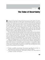
not. The basic concept is outlined in graphical forms in Figure 4.1, which
has been adapted from the authors’ work.
Once a firm initiates a new product or service development program, it
faces a significant degree of technical or private uncertainty that will only be
resolved over time as the product or service is being developed. Initially, the
firm is also uncertain about what level of performance features the final
product or service will meet. Management and engineers or marketing per-
sonnel are likely to have some beliefs, though, as to the probability to reach
different levels of performance of the product or of the service to be imple-
mented. The product or service then enters a market that may either be
highly sensitive to performance criteria (scenario A) or minimally sensitive to
performance criteria (scenario B). In scenario A, incremental increases in
product or service performance are rewarded by large increases in payoffs.
106 REAL OPTIONS IN PRACTICE
Time
Technical

Uncertainty
Market Requirements
Product Performance
Probability Payoff
A
B
Probability
Payoff
A
B
FIGURE 4.1 Market variability reduces option value. Source: Huchzermeier and Loch
In scenario B, even significant improvements of product or service perfor-
mance criteria will only yield incremental additional payoffs.
The degree of technical or private uncertainty, the degree of product
performance uncertainty, and the degree of market requirement uncertainty
drive the shape of the ultimate payoff function. A high market uncertainty
(scenario A) will result, everything else remaining equal, in a much more un-
certain and volatile payoff function. With a very small probability, manage-
ment can expect a significant payoff; with much higher probabilities, the
expected payoff for scenario A levels off very quickly. On the contrary, the
payoff function of scenario B with little market requirement uncertainty is
much less volatile. With a higher probability, management can expect to re-
alize the maximum payoff, and with increasing certainty there is only a
small decline in the expected payoff.
We will now model market variability uncertainty in a binomial model.
Let’s assume that a pharmaceutical company has a portfolio of four differ-
ent pre-clinical products for different disease indications. For each product,
scientists and clinical researchers can define reasonably well five classes of
distinct product performance categories, designated 1 to 5, by looking into
efficacy, side-effects of the compound, interaction with other drugs likely to

be taken by the same patient population, convenience in administering it for
patients and doctors, and ultimately the cost-benefit profile. Scientists and
clinicians can further predict with reasonable confidence for each product
the likelihood of meeting each of the product performance criteria. The four
products address different disease indications. In each disease indication the
therapeutic market looks different. Specifically, in each market, the future
acceptance and ultimately the market share of the product will display dis-
tinct and different sensitivities to the product performance of the future
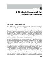
drug. The various scenarios are depicted in Figure 4.2.
For example, in an already crowded market of hypertensive drugs, in-
cremental product performance will not impact much on overall market
share. However, if the product turns out to be very superior and offers sig-
nificant cost savings, it can capture a significant share of a big market (prod-
uct scenario 1). The second product targets a market where there is no
satisfactory treatment yet. The technical uncertainty of developing the prod-
uct may be higher, but the market payoff function is largely independent of
incremental improvement in product performance along the categories out-
lined above. The product will capture a significant market once its clinical
efficacy is proven and it is approved; further improvements along any of the
other product performance categories will have only incremental if any ef-
fect on market share (product scenario 2). The volatility between the best
and the worst product performance category is very small. Yet another
The Value of Uncertainty 107
compound targets a market where any incremental improvement in the side-
effect profile and drug-interaction profile is likely to help capture a signifi-
cant fraction in a currently fragmented market, while further improvements
are unlikely to result in major increases in market share (product scenario 3).
Finally, let’s assume there is a fourth product where each step in product im-
provement will result in incremental steps in more market share (product
scenario 4).

The market requirement variability is clearly distinct for each product
(Figure 4.2). We will now examine how this plays out in the option valua-
tion. In order to get a good understanding of the isolated effect of market re-
quirement variability on the option value of each of these investment
projects, we assume initially that all other key drivers of option value, in-
cluding future asset value as well as private or technical uncertainty to de-
velop the four different products are the same. We will in a later chapter
(Chapter 7) relax these assumptions and vary the technical risk as well as the
market size to find the right investment decision for this product portfolio.
We also assume for each product and for each product feature the same
technical probability of success of 20%. In other words, our pharmaceutical
firm is equally capable of developing all five product features for all four
products. As a result, we eliminate any effect that technical uncertainty may
have on actually succeeding in product development.
Product 1 has the largest variance for market requirements: incremental
product improvement leads to significant increases in market share. Product
108 REAL OPTIONS IN PRACTICE
0%
012345
10%
20%
30%
40%
50%
60%
70%
80%
90%
100%
Product Scenarios

Market Requirement Probability (%)
Feature 1
Feature 2
Feature 3
Feature 4
Feature 5
FIGURE 4.2 Product market variability scenarios
2 has the smallest market requirement variability: small product improve-
ments will have only little impact on overall market share. Product 3 has less
market requirement variability than Product 4. How does the market vari-
ability affect the value of the option on the drug development program? We
work with the same assumptions as in Chapter 3 regarding costs, time to de-
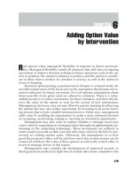
velopment, and overall technical risk. Figure 4.3 summarizes the binomial
asset tree.
The expected value at time of launch is different for each of the prod-
uct scenarios and reflects the assumptions on market variability. The ex-
pected value at the time of launch is determined by both market uncertainty
as well as market requirement variability. Figure 4.4 summarizes the steps
The Value of Uncertainty 109
Pre-Clin
Phase II
Phase III
NDA
Future
V
max
Best Case = 520m
eV
V
min

Worst Case = 24m
Phase I
1 year
3m
1 year
5m
2 years
10m
2 years
20m
1 year
6m
0.6
0.4
0.6
0.4
0.5
0.5
0.75
0.25
0.9
0.1
Now
Expected Values:
Scenario 1: 91.91m
Scenario 2: 234.89m
Scenario 3: 156.76m
Scenario 4: 130.21m
FIGURE 4.3 The binomial asset tree of the compound option under market variability
Market Uncertainty

Best
Case
520m
Worst
Case
24m
Expected
Market
Value
255m
50%
50%
EMV
•
(q
1
•
MS
1
+ q
2
•
MS
2
+ q
3
•
MS
3
+ q

4
•
MS
4
+ q
5
•
MS
5
)
Expected
Product
Value
Market Variability
FIGURE 4.4 How to calculate the asset value under market uncertainty
taken to calculate the expected product value at the time of launch for each
product.
The expected market value is based on managerial assumptions of the
best case and worst case scenario and the probability assigned to each to
occur, amounting in our example to $255 million. This figure also went into
the initial compounded option analysis of this drug development program in
Chapter 3. To arrive at the expected product value at the time of launch we
multiply the expected market value (EMV) by the technical probability q
x
of
implementing the product feature that will allow capturing the market share
assigned to this product feature (MS
x
). This gives us the expected product
value (EPV) at the time of launch for each of the four products.

For example, for product 1, the expected product value is:
EPV
1
= $255 million
•
(0.2
•
8 + 0.2
•
12 + 0.2
•
22 + 0.2
•
38 + 0.2
•
100)
= $91.91 million
For product 1, there is a 20% chance for each to achieve incremental prod-
uct improvements that will help to capture 8%, 12%, 22%, 38%, and ulti-
mately 100% of the market. This translates into an expected value at launch
of $91.91 million. For product 2, however, each improvement step with a
20% chance of success will advance the overall market share from 85% to
88%, 92%, 95%, and ultimately 100%, yielding an expected market value
of $234.89 million. We calculate the EPV for each product at the time of
launch. The maximum asset value at the time of launch for each product is
$520 million, assuming that all product features are met and that the full
market can be captured. Likewise, the minimum asset value assumes that there
is no market variability, and the minimum market value will be captured,
that is, $24 million at the time of launch and zero at any time prior to the
time of launch.

As in our basic compound option model, we take the expected product
values back to the pre-clinical stage of development, applying the same
probability of success as before (Chapter 3). We calculate p for each prod-
uct scenario and stage of development as before (p = [(1 + r)
•
EPV – V
min
] /
[V
max
– V
min
]) and then determine the value of the call for each stage under
each product scenario. Figure 4.5 depicts the results and also shows again,
for comparison, the value of the option for the product, ignoring market re-
quirement variability (dashed line and solid symbol).
The fundamental insight provided by this analysis is that market require-
ment variability reduces the value of the investment option: the higher the vari-
ability, the lower the option value. That effect is most pronounced when a
110 REAL OPTIONS IN PRACTICE
comparison is made between the option values of product 1 and product 2.
The highest option value is seen in the absence of market variability.
This notion is contrary to the general assumption that increasing uncer-
tainty increases the value of your option. It points to the importance of dif-
ferentiating the sources of uncertainty and their value on the asset and hence
on the option. While increased market payoff uncertainty increases the value
of the option, market requirement variability, as previously pointed out by
Huchzermeier and Loch, does not.
In essence, the more a given set of product features drives diverse pay-
offs, the smaller the likelihood of reaching a certain fraction of the market

becomes. For example, with 60% probability, product 1 will meet three
product hurdles and thereby have 22% of the market. With the same prob-
ability, product 2 reaches three product hurdles, but by then already cap-
tures 92% of the market.
The analysis also promotes another question: How sensitive is the value
of the option to a change in market variability when it is at the money, for
example, at the pre-clinical stage of drug development, compared to when it
is deep in the money, for example, at launch? Clearly, Figure 4.5 suggests
that the absolute impact of market variability uncertainty increases sharply
as the four product options move deeper into the money as they progress
successfully through the development stages.
The Value of Uncertainty 111
0
50
100
150
200
250
300
Pre-Clin Phase I Phase II Phase III FDA Filing Launch
Development Stage
Value of the Option ($m)
Product 1
Product 2
Product 3
Product 4
No Market Variability
FIGURE 4.5 Value of the compound option under market uncertainty
Figure 4.6 examines this in more detail. It displays the change of option
value under increasing market variability as a percentage of base-line value

in the absence of market variability for the investment opportunity. Shown
are the data for the option value in the pre-clinical stage, when the option is
either out of the money or at the money, as well as for the launch stage,
when the option is deep in the money. The four product scenarios are
arranged on the x-axis in such a way that the variability decreases from left
to right, that is, highest for product scenario 1 and lowest for product sce-
nario 2.
The data suggest that market variability consistently has a greater rela-
tive impact on the percent change of option value for an option at the money
(product in pre-clinical stage, round symbols) compared to an option deep
in the money (product at launch, square symbols). As market uncertainty de-
clines, moving from left to right on the x-axis, that differential also declines.
This insight is important in developing an understanding as to when
market uncertainty becomes an important driver of option valuation. Such
an understanding in turn becomes important for management in defining the
conditions when there is value in resolving market variability uncertainty,
that is, by making investments in active learning. For an investment option
that is deep in the money, resolving market uncertainty is not so critical. For
an option that is at the money, reducing the uncertainty surrounding market
requirement variability is much more crucial. If management believes that
market product requirements display little volatility (product scenario 4),
112 REAL OPTIONS IN PRACTICE
0%
10%
20%
30%
40%
50%
60%
70%

80%
90%
100%
1432
Product Scenario
Option Value as % of Base-Line
Pre-Clinical
Launch
FIGURE 4.6 Loss of option value with increasing market uncertainty
there is little value in resolving any residual uncertainty for options that are
either deep in the money or just at the money. On the other hand, if market
requirement variability is perceived to be very high, then management may
want to invest resources in learning and defining the market variability,
specifically for investment options that are only at the money.
REAL CALL OPTIONS WITH
UNCERTAIN TIME TO MATURITY
Real options, other than financial options, often suffer from the random na-
ture of the time to maturity of an investment. It is unclear for projects of a di-
verse nature how long it may take to complete them so that they create
revenue streams for the organization. It is equally unclear, for the majority of
real asset values, how long they will generate a profitable revenue stream, with
potential competitive entry or future technology advances not yet resolved.
In the introductory chapter we saw that some of the value of a financial
option is derived from the time to maturity: the farther out the exercise date
is the more valuable the option becomes, everything else remaining equal.
For a real call option, that is not true. The farther out the time to maturity
is, the farther away the future cash flows generated by the asset to be ac-
quired are, and hence the smaller the current value. This simply acknowl-
edges the time value of money. In addition, a key difference between real and
financial options is that financial options are monopoly options, while real

options are often shared. Competitive entry may prematurely terminate a
real option. Further, for real options, we often do not know exactly what the
time to maturity is, as development times to implement and create real assets
are uncertain.
Some of the time uncertainty is technical or private in nature. For ex-
ample, for a new product development program, management will only have
an estimate as to how long it may take for scientists and engineers to come
up with the first prototype if all goes smoothly. Bumps that delay the devel-
opment are likely, and potentially less likely are “eureka” moments that ad-
vance and speed up the development.
What effect does uncertain time to maturity have on the option value?
How sensitive is the value of a real call option to time volatility? To draw
the comparison to a financial option: This decision scenario represents a call
option on a dividend-paying stock; the call owner obtains the dividend only
when he exercises the option and acquires the stock. While the advice to
American call owners is never to exercise, this guidance changes if the option
The Value of Uncertainty 113
is on a stock that pays a dividend. The best time to exercise an American call
option on a dividend-paying stock is the day before the dividend is due.
Maturity, in the world of real options, is private, and there is no hedge.
The closest we come in financial options to the problem of unknown matu-
rity is an American option with random maturity. Here, the value of the op-
tion is always smaller than the value of the weighted average of the standard
American call, an insight Peter Carr gained in his 1998 paper.
2
The intuition
behind Carr’s conclusion is that an American option with random maturity
really is nothing other than a portfolio of multiple calls with distinct matu-
rities. The owner of the option will exercise the entire portfolio at the same
exercise time, and therefore the value of the call must be less than for a ran-

domized option, while the critical value to invest is higher.
The random maturity lowers the value of the option and reduces the
trigger value.
3
In fact, as time to maturity becomes highly uncertain, the crit-
ical threshold to invest approaches the level an NPV analysis would yield,
killing in effect the option value of waiting. The size of the impact of uncer-
tain time of maturity will depend on the distribution of maturity, mean, and
variance. The higher the volatility, (that is, the more uncertain the time to
maturity is), the more the lower and the upper border of the option space
converge, until they finally collapse at the NPV figure. For real options, the
uncertainty of the maturity time stems from a variety of sources, the most
obvious being competitive entry that kills significant option value.
Assume that management has an opportunity to invest $100 million in
a new product line that has a probability of 50% to create cash flows with
a present value of $500 million for the expected lifetime at the time of prod-
uct launch. In the worst case scenario, the present value of those revenue
streams at time of product launch will be only $200 million. Management
envisions four scenarios as to the time frame necessary to complete the de-
velopment of its new product line, as summarized in Figure 4.7.
Please note that we do not include in the analysis that the time to ma-
turity will also affect the revenue stream: the sooner the product reaches the
market, the more cash flow will be generated. To strictly investigate the ef-
fect of time uncertainty we assume that the amount of cash flow generated
will not change as a function of the timing of product launch. Table 4.1
summarizes the basic parameters to calculate the call option. We give the
value of the call assuming a certain time to maturity of four years.
As time is uncertain, there is for each of the four scenarios a distinct
probability to complete the program and launch the product at any given
time. For example, for scenario 1, the probability to complete after 2 years,

3 years, 4 years, 5 years, or 6 years is 20% for each. On the contrary, for sce-
nario 2, the likelihood to complete the project in 2 years is only 3%, while
114 REAL OPTIONS IN PRACTICE
at a probability of 85% the product will be completed after four years. To
acknowledge uncertainty of time to maturity in the calculation of the option
value for the four different scenarios, we need to incorporate the probabil-
ity function of completion when discounting the option value to today’s
The Value of Uncertainty 115
0
1
2
3
4
5
6
7
0 20406080100
Probability of Completion (%)
Year of Completion
Scenario 1
Scenario 3
Scenario 4
Scenario 2
FIGURE 4.7 Time to maturation scenarios for a new-product development program
TABLE 4.1 The basic call option
parameters—without time uncertainty
Basic Option Parameters
WACC 13.50%
Risk-Free Rate 7%
q 0.5

Expected Value 350
Max Value 500
Min Value 200
Cost 100
p 0.581666667
t (years) 4
Call 185.70
time. The formula below shows the calculation: The probability q to com-
plete the project for each time scenario t
2
to t
5
goes into the denominator to
acknowledge the expected time to completion when discounting the option
value:
This gives us the following results for the call option for each time scenario
as summarized in Table 4.2.
There is a substantial difference in option value between the four sce-
narios investigated. This is to a large degree explained by the fact that the ex-
pected time to completion for each scenario is different, thus yielding
significant sooner or significant later cash streams that will alter the option
value simply because of the time value of money. Table 4.3 summarizes the
expected time to completion for each scenario.
By fixing the expected time to completion to four years but varying the
variance, we eliminate the effect of the time value of money and see the ef-
fect of time volatility. Figure 4.8 depicts on the left panel four different time
scenarios, all of which have an expected time to completion of four years,
and on the right panel the corresponding value of the call options.
The effect of increasing the volatility of time to maturity is small but no-
ticeable. The value of the call option is highest in the absence of time uncer-

tainty (scenario 5) and lowest if the variance of the time to maturity ranges
between 1 and 7 periods (scenario 4). Note that the analysis has not included
the effect of uncertain time to maturity on the opportunity cost of capital.
However, the analysis also shows that time uncertainty has a significant ef-
C
pV p V
qrqrqrqr
x
tx tx tx tx
=
+−
++ ++ ++ +
⋅⋅
⋅⋅⋅
max min
()
() () () ()
1
1111
2
2
3
3
4
4
5
5
116 REAL OPTIONS IN PRACTICE
TABLE 4.2 The option value under time uncertainty
Value of the Call Option

Timing Scenario 1 2 3 4
Call Value ($ m) 184.40 185.90 212.48 159.68
TABLE 4.3 Expected time to completion under four product
development scenarios
Expected Time to Completion (years)
Timing Scenario 1 2 3 4
Expected Time 4.00 3.98 2.63 5.37
fect on option value only if it alters the expected time to completion or ma-
turity time.
Time to maturity not only impacts on option value, but also on the crit-
ical cost to invest: The farther out the cash flow stream, the smaller its
today’s value, and hence the sooner the option is out of the money. The
higher the uncertainty as to when cash flow will materialize, the lower in-
vestment costs should be not to move the option out of the money. Similarly,
the higher the uncertainty surrounding time to maturity or project completion,
the higher the critical asset value needs to become to justify investing the
anticipated costs without moving the option out of the money. Figure 4.9
shows for the five different timing scenarios and an expected asset value of
$350 million the critical cost to invest. If management were to invest more
than the critical cost, the investment option would move out of the money.
The Value of Uncertainty 117
1
2
3
4
5
6
7
0% 50% 100%
Probability (%)

Time to Completion (Years)
Scenario 1
Scenario 2
Scenario 3
Scenario 4
Scenario 5
182
183
184
185
186
123 4 5
Time Scenarios
Option Value ($m)
FIGURE 4.8 Time uncertainty and option value
283
284
285
286
12345
Time Scenarios
Critical Cost to Invest ($ m)
FIGURE 4.9 The critical cost to invest under time uncertainty
In the absence of time to maturity uncertainty (scenario 5), the critical
cost to invest is highest. As the volatility of timing increases, the critical cost
that management should be prepared to invest in the project declines. It is
lowest for scenario 4, which has the highest time to completion volatility.
Previously, when looking at the effect of market variability, we saw
how the sensitivity of the option value changes depending on whether the
option is at the money or deep in the money. We will now investigate the

sensitivity of the call option to time uncertainty depending on whether the op-
tion is at the money or in the money. In the example given in Figure 4.10, we
reduce the maximum asset value from $500 million (see Table 4.1) and
allow it to vary between $200 million and $300 million. We first calculate
the value of the option for this range of best case scenarios under each time
uncertainty scenario. The results are summarized in Figure 4.10.
The time uncertainty scenarios are arranged in such a way that the time
volatility declines from left to right. At a maximum asset value of $200 mil-
lion, the option is just at the money for all time uncertainty scenarios; at a
maximum asset value of $300 million, the option is deep in the money. For
all best case market payoff assumptions, a decline in time volatility (moving
118 REAL OPTIONS IN PRACTICE
0
5
10
15
20
25
30
35
40
45
413 25
Timing Scenario
Option Value ($m)
Maximum Value of 200
Maximum Value of 210
Maximum Value of 250
Maximum Value of 300
FIGURE 4.10 Option value sensitivity to time uncertainty for at- and in-the-money

options
from left to right on the x-axis) appears to do little to the overall option
value.
We now examine the effect of time uncertainty in more detail by look-
ing at the change in option value for each of the future payoff scenarios as a
percentage of the base-line option value under no time uncertainty (scenario
5). Figure 4.11 summarizes the data.
High time uncertainty changes the option value significantly for an op-
tion that is at the money. For example, for a maximum future payoff of
$200 million the option value under high time uncertainty in scenario 4 is re-
duced by 34% compared to the option value under no time uncertainty. For
a less volatile scenario, such as scenario 2, the value difference for an at the
money option is only 4.4%. As the expected future payoff increases and the
option moves more and more into the money, the option value becomes less
sensitive even to significant time uncertainty. At a future payoff of $300 mil-
lion, with the option deep in the money, even high time uncertainty (scenario
4) does little to change the value of the option. The option value under high
time uncertainty (scenario 4) is reduced by 2.2% compared to the conditions
The Value of Uncertainty 119
0%
10%
20%
30%
40%
4132
Timing Scenario
Option Value as Percentage of Base-Line
Maximum Value of 200
Maximum Value of 210
Maximum Value of 250

Maximum Value of 300
FIGURE 4.11 Option value loss under time uncertainty for at- and in-the-money
options
without time uncertainty. As time volatility declines, moving on the x-axis
from left to right, its impact on option value becomes less and less material,
irrespective as to whether the option is at the money or deep in the money.
What is the implication for management? Time uncertainty becomes
more critical to understand and control as the option is at the money than
for a call option deep in the money. However, time uncertainty is not very
material as long as the expected time to maturation does not change. Man-
agement may want to invest in learning and controlling time uncertainty for
call options at the money but should be less inclined to do so for call options
deep in the money, unless the expected time to maturity can be shortened to
capture the time value of money and/or some preemptive value.
REAL PUT OPTIONS WITH UNCERTAIN
TIME TO MATURITY
Uncertain time to maturity may also refer to the length of time a real put op-
tion is viable for the holder of an asset for which market conditions deteri-
orate. For example, the sudden entry of a competitor may terminate or
significantly diminish the current cash flow from an existing asset prema-
turely or alter its value considerably. This situation is comparable to an
American put on a dividend-paying stock.
The company receives a constant dividend, namely, the cash flows gen-
erated by the asset. However, it is unclear when the asset may move out of
the money and the revenue stream dies off or reaches such a low level that
the operation becomes unprofitable. How do we value real put options
when time to maturity is unknown, or at least very uncertain?
Let’s start with a simple example. Management owns an asset that cre-
ates $200 million in value. Management believes that a competitive entry
will happen, but the time frame is uncertain. If it happens, the maximum

value to be generated from the existing asset may still stay at $200 million
in value in the best case scenario, or drop to $30 million in the worst case
scenario. Each scenario is equally likely (i.e., q is 50%). Management can
abandon fixed assets related to the product against a salvage price of $130
million as soon as a competitive entry becomes certain. This price reflects
management assumptions about the outstanding value of the fixed assets
over their remaining lifetime. What is the value of this put option?
Initially, we determine the put option value by assuming that the antic-
ipated competitive entry and decline will happen with certainty four years
from now. The exercise price for the put is today’s value for the revenues
foregone over the remaining lifetime of the asset. The value of the underly-
120 REAL OPTIONS IN PRACTICE
ing asset is the salvage price management expects to receive when selling the
asset. In this scenario we are valuing a put with a determined asset value but
uncertain exercise price. The equation to calculate the value of the put is:
with S
v
denoting the salvage value of $130 million and K
max
and K
min
denot-
ing the maximum and minimum revenue stream foregone when exercising
the put option on the asset, equivalent to the exercise price. Table 4.4 shows
the basic put option parameters and the put value for the basic scenario.
We now introduce uncertainty to the time of maturity. We use the same
assumptions as for the call option in the previous section. These assumptions
reflect management’s beliefs as to when the drop in asset value will occur.
These sets of assumptions yield, as shown before, a disparate set of expected
times to maturity, shown on the left panel of Table 4.5, and a mean time to

maturity set fixed at four years (mean) but with smaller or larger variance.
To acknowledge uncertainty of the time to maturity we calculate the value
of the put option—as was done before for the call option—by incorporating
the probability q for each time scenario t
2
to t
5
using the following formula:
Using this formula, we arrive at the following values for the put option
under the different timing conditions, summarized in Table 4.5.
P
SpK pK
qrqrqrqr
v
tt t t
=
−⋅ +−⋅
++ ++ ++ +
⋅⋅⋅
[()]
() () () ()
max min
1
1111
2
2
3
3
4
4

5
5
P
SpK pK
r
v
t
=
−⋅ +−⋅
+
[()]
()
max min
1
1
The Value of Uncertainty 121
TABLE 4.4 The basic put option
parameters—without time uncertainty
WACC 13.50%
Risk-Free-Rate 7%
q 0.5
Expected Value 115
Max Cost K 200
Min Cost K 30
Salvage Value 130
p 0.54735
t (years) 4
Put $5.30
The way this scenario is set up for the put option, both the asset value
(that is, the salvage value) and the exercise price (that is, the present value of

the revenue stream) are subjected to the time uncertainty, as management will
make the decision to abandon the project at the time point of competitive
entry, and that time point is subject to uncertainty. This set up is different from
the previous example, which looked at the value of the call option under time
uncertainty. There, the timing of the exercise price (that is, the commitment of
the investment costs K) was fixed and not subject to uncertainty.
This explains why we do not see for this put scenario the same degree of
change in value of the put, as the expected time to maturity changes between
2.63 and 5.37 years (left panel, Table 4.5 above). This reflects that time un-
certainty in this scenario is the same for both asset value as well as exercise
price, and is therefore perfectly correlated. A positive correlation, as we
have discussed in Chapter 2, provides a hedge but reduces overall volatility
and thereby the option value. As with the call option, we note for the put op-
tion that the value decreases the farther out the time to maturity lies. We fur-
ther see qualitatively that uncertainty in the timing of expiration has the
same effect on the put option as on the call option: The more certain the
time is (scenario 5), the higher the value of the put option; the more volatile
the time is, the lower the value of the put option (scenario 4). The quantita-
tive difference, however, is less pronounced for the put option in the chosen
set up than for the call option in the previous example as cost and asset
volatility are perfectly correlated.
We will now introduce an example in which the salvage price is fixed
today but the exercise price is subjected to uncertain time to expiration.
Imagine that management has the option to abandon the asset today against
a salvage price of $130 million. Management has some beliefs as to when
competitive entry will occur, leading to the projected decline in asset value,
122 REAL OPTIONS IN PRACTICE
TABLE 4.5 The value of the put option under time uncertainty
Expected Time of Maturity Expected Time to Maturity
(years) (years)

1234 1 2345
4.00 3.98 2.63 5.37 4.00 4.00 4.00 4.00 4.00
Value of the Put Option Value of the Put Option
1234 1 2345
5.28 5.31 5.80 4.82 5.28 5.30 5.29 5.27 5.30
but there is uncertainty about the exact timing. As done previously with the
call option example, we will ignore the effect that uncertain timing has on
the revenue stream to separate out market uncertainty from timing uncer-
tainty in the valuation of this put option.
The value of the put option for this set up is calculated using the fol-
lowing equation:
Table 4.6 summarizes the basic option parameters as well as the value of the
put option for a time to expiration fixed at four years.
We now study the effect of uncertain time to maturity by expanding the
formula for the put for this set up, as shown in the following equation:
Management’s beliefs as to the timing scenarios are the same as shown
for the call option, which gives rise to the following put option values, sum-
marized in Table 4.7. As we have seen for the value of the call option under
uncertain time to maturity, we also see for the put option in this set up that
PS
pK p K
qrqrqrqr
v
tt t t
=−
+−
++ ++ ++ +
⋅⋅
⋅⋅⋅
max min

()
() () () ()
1
1111
2
2
3
3
4
4
5
5
PS
pK p K
r
v
t
=−
+−
+
⋅⋅
max min
()
()
1
1
The Value of Uncertainty 123
TABLE 4.6 The basic put option
parameters—with fixed expected time
to maturity

Basic Put Option
WACC 13.50%
Risk-Free-Rate 7%
q 0.5
Expected Value 115
Max Cost 200
Min Cost 30
Salvage Value 130
p 0.5474
t (years) 4
Put $36.13
the value of the option is most sensitive to changes in the expected time to
expiration. However, contrary to what we have seen with the call option,
the value of the put option in this set up declines as the expected time to ex-
piration shortens.
For example, with an expected time to expiration of 2.63 years, the
value of the put option is $27.33 million, while for an expected time to ex-
piration of 5.37 years, the value of the put option is $44.68 million. For a
short expected time to maturity the value of the asset is higher simply be-
cause of the time value of money. So, giving it up against the salvage price
implies a smaller payoff. As time moves on, today’s value of the asset de-
clines, and the payoff from salvage at a price fixed today goes up. What is
the intuition? Remember, we assume the overall cash flow that management
expects still to be generated by the fixed assets to be at best $200 million and
at worst $30 million. It is unclear, though, whether this cash flow will be
generated over an expected time of maturity of 2.63 years (scenario 3) or
over 5.37 years (scenario 4). In scenario 3, the time value of revenues fore-
gone today, at the time management contemplates salvaging the fixed assets
against $130 million, is $102.67 million; in scenario 4 it is $85.32 million.
The value of abandoning the fixed assets today is smaller if revenues fore-

gone can be cashed out quickly, while an asset with a protracted but low
revenue stream has a higher abandonment option value.
Also, for this put option set up, the effect of time volatility is opposite
that which we saw for the call option, as shown in the right-hand panel of
Figure 4.8. Remember that here the expected time to expiration is fixed at
four years, but the volatility varies. With certain time to maturity of 4 years
(scenario 5, right-hand panel), the value of the put is lowest. As volatility of
timing increases, the value of the put also increases. It is highest for scenario
4, which captures the most volatile timing assumptions. The call option, as
we have seen before, behaves in an opposite manner: the less volatile the tim-
ing to maturity becomes, the more the call option increases in value.
124 REAL OPTIONS IN PRACTICE
TABLE 4.7 The value of the put option under increasing time volatility
Expected Time of Maturity Expected Time to Maturity
(years) (years)
1234 12345
4.00 3.98 2.63 5.37 4.00 4.00 4.00 4.00 4.00
Value of the Put Option ($m) Value of the Put Option ($m)
1234 12345
36.55 36.06 27.33 44.68 36.55 36.20 36.34 36.76 36.13
TECHNOLOGY UNCERTAINTY
Many firms not only have to question the timing and sizing of their invest-
ments in new-product development but also examine carefully in what tech-
nology to invest at what point in time, given that technologies in most
industries undergo rapid advancements. A computer maker will have to con-
sider which technology to implement in his latest models and whether he
may be better off waiting another year or two, until an even better technol-
ogy becomes available for his products. On the other hand, discoveries hap-
pen randomly, and regularly there is little or no correlation between the
resources put into research and the creation of an asset that will result in a

profitable cash flow. As Weeds points out:
4
“When the firm exercises its op-
tion to invest in research it gains a second option, that of making the dis-
covery itself, whose exercise time occurs randomly rather than being a single
date chosen explicitly by the firm.” This situation of technical uncertainty
may provide an additional incentive to defer an investment.
Let’s examine how such a scenario can be modeled in a binomial option
model. We assume that a firm faces the decision either to adopt an existing
technology today for its next generation of products, or to wait until the new
technology arrives at a yet unknown time. Management assumes that the
firm can use either the existing technology 1 or a future technology 2 whose
arrival date is uncertain. Once the current technology 1 is adopted, the firm
foregoes the option to adopt any new technology for a period of three years.
This time frame reflects management’s assumptions about development
times as well as product life expectancy in a competitive market.
Technology 1 is already developed and in place; there is no technical
risk associated with the implementation of technology 1. Technology 2,
however, still needs to be implemented and there is some uncertainty as to
whether the firm will be able to do so.
For now we do ignore the competitive environment for this decision, but
we will relax this assumption later. Whether management is better off to im-
plement technology 1 now or to wait for technology 2 is likely to be influ-
enced by management’s beliefs about the following parameters:
The importance of the new technology for sustaining or expanding ex-
isting market share.
The costs and time frame of implementing the new technology.
The private probability q of being successful in implementing the new
technology.
The opportunity cost foregone due to waiting for the arrival of technol-

ogy 2 if technology 1 is not implemented.
The Value of Uncertainty 125
We will provide a binomial model that allows incorporating and varying all
these parameters. Figure 4.12 shows the binomial framework.
Management initiates an intensive discussion internally with engineers,
scientists, and the product development team, as well as the marketing team,
and also spends resources on primary and secondary market research and
some competitive intelligence to better define the environmental conditions
for this investment decision. As a result of these initiatives, the company
comes up with the following set of consensus assumptions.
Management assumes three different probability distributions to predict
the arrival of technology 2. At yet uncertain costs, management will have the
option to acquire technology 2 (node 1). The probabilities of success in im-
plementing the technology and integrating it in the new product are still ill de-
fined (node 2 and 3). However, if the company succeeds in implementing
technology 2, there are three distinct probability distributions that depict the
future market payoff (node 4 and 5). For the currently available technology
1, management believes that a product containing technology 1 will be less
competitive and less likely to gain significant market share, but will also be
cheaper as well as quicker to develop and bring to market. Management be-
lieves that it will cost $50 million to implement technology 1, that there will
be no technical risk (technology probability of 100%; q
6
= 1), and that it will
be able to develop and launch the product in one year. Management assumes
three basic scenarios to reflect product penetration using the currently avail-
126 REAL OPTIONS IN PRACTICE
Probability
Payoff
Technology 2

Arrival
1
2
3
– K?
– K?
q
2
= ?
q
3
= ?
q
7
= 0
q
6
= 1
4
9
5
7
Time
Probability
Implementation
Implementation
6
8
Probability
Payoff

FIGURE 4.12 The binomial asset tree for technology uncertainty
able technology 1, each of which is equally likely (q = 0.333). These scenar-
ios are driven by other uncertainties such as the competitive environment and
overall global economic situation that affect demand. Management also as-
sumes that peak market penetration will be reached in year 6 and decline
thereafter. The overall market size lies somewhere between $500 million in
annual revenue as the best case scenario and $200 million in revenue as the
worst case scenario for the product. The probability q for the best case sce-
nario is 0.7, and 0.3 correspondingly for the worst case scenario. Table 4.8
summarizes management’s assumptions about market penetration scenarios
for a product containing technology 1 and future revenue streams.
The expected value generated from the asset in year 1 is the present
value of these revenue streams weighted for their probability of occurrence
(that is, 0.7 for the best case (BC) scenario, 0.3 for the worst case (WC) sce-
nario, and 0.333 for each of the market penetration scenarios (S1, S2, S3).
V
exp
= [ 0.7
•
(0.333 BC – S
1
+ 0.3333 BC – S
2
+ 0.333
•
BC – S
3
) + 0.3
•
(0.3333 WC – S

1
+ 0.3333
•
WC – S
2
+ 0.33333
•
WC – S
3
)]
The Value of Uncertainty 127
TABLE 4.8 Basic market uncertainties: Penetration scenarios and future revenue
stream scenarios for a product with technology 1
Market Penetration
Time of Entry 1 2 3
(years) (%) (%) (%)
1531
2852
31584
420108
5271510
Revenue Stream
Scenarios Year 2 Year 3 Year 4 Year 5 Year 6 q
Best Case Scenario
1 25 40 75 100 135 0.333
2 15 25 40 50 75 0.333
3 5 10 20 40 50 0.333
Worst Case Scenario
1 10 16 30 40 54 0.333
2 6 10 16 20 30 0.333

3 2 4 8 16 20 0.333
The maximum asset value is derived from assuming that the overall
market size will be the best case scenario (i.e., $500 million); the minimum
asset value correspondingly derives from assuming that the worst case mar-
ket size will materialize. For each, the revenue streams for the different sce-
narios with their corresponding probability of occurrence (0.3333) will be
added up. These assumptions translate into the following parameters, shown
in Table 4.9 for the call option on investing into technology 1, assuming
there is no risk of technical failure.
For the arrival of technology 2, management envisions three different
timing scenarios. Those assumptions are summarized in Figure 4.13, with
the time of arrival on the x-axis and the probability of arrival on the y-axis.
The probability of actually succeeding in implementing the new technology
for its product is thought to range between 50% and 85%.
Management further assumes that the overall market size for the prod-
uct, $500 million in the best case scenario and $200 million in the worst case
scenario, will be independent of its decision to implement technology 1 or
technology 2. Management also assumes that the probability of reaching the
best case scenario is 70%, while the probability for the worst case scenario is
128 REAL OPTIONS IN PRACTICE
TABLE 4.9
The call option value for
technology 1 in the absence of private risk
Probability of Technical
Success 100%
Expected Value $90.96
V
max
$129.95
V

min
51.98
p 0.58167
Call $20.60
0%
20%
40%
60%
80%
100%
012345
Probability of Arrival
Time of Arrival (Year)
Scenario 1
Scenario 2
Scenario 3
FIGURE 4.13 New technology arrival scenarios
30%. However, the market penetration is thought to be more aggressive for
a product with technology 2, yielding ultimately a higher revenue stream.
There is no expectation that the market potential will expand with the new
technology. Table 4.10 summarizes managerial assumptions and the antici-
pated revenue streams resulting from launching a product with technology 2.
The expected value generated from the asset in year 2 is—as was out-
lined above for the technology 1 product—the present value of these revenue
streams weighted for their probability of occurrence (that is, 0.7 for the best
case scenario, 0.3 for the worst case scenario, and 0.333 for each of the mar-
ket penetration scenarios).
V
exp
= [ 0.7

•
(0.333 BC – S
1
+ 0.3333 BC – S
2
+ 0.333
•
BC – S
3
) + 0.3
•
(0.3333 WC – S
1
+ 0.3333
•
WC – S
2
+ 0.33333
•
WC – S
3
)]
The expected value of the future asset to be generated by technology 2
is in addition a function of the timing and probability of technology 2 ar-
rival, the technical probability to succeed in implementing it, and the future
market payoff scenarios. We multiply the expected value as calculated above
The Value of Uncertainty 129
TABLE 4.10 Basic market uncertainties: Penetration scenarios and future revenue
stream scenarios for a product with technology 2
Market Penetration

Time of Entry 1 2 3
(years) (%) (%) (%)
21553
325105
435158
5452512
6503518
Revenue Stream
Scenarios Year 2 Year 3 Year 4 Year 5 Year 6 q
Best Case Scenario
1 75 125 175 225 250 0.333
2 25 50 75 125 175 0.333
3 15 25 40 60 90 0.333
Worst Case Scenario
1 30 50 70 90 100 0.333
2 10 20 30 50 70 0.333
3 6 10 16 24 36 0.333