Advanced Maya Texturing and Lighting- P5 potx
Bạn đang xem bản rút gọn của tài liệu. Xem và tải ngay bản đầy đủ của tài liệu tại đây (3.26 MB, 30 trang )
99
■ CHAPTER TUTORIAL: LIGHTING A FLICKERING FIRE PIT WITH SHADOWS
Chapter Tutorial: Lighting a Flickering Fire Pit with Shadows
In this tutorial, you will create a fire with soft, flickering shadows (see Figure 3.29).
You will use Paint Effects fire with a volume, ambient, and directional light.
Fir e pi t m o d e l co ur te sy oF Kr is t en sc al l i on
Figure 3.29 Fire created with a Paint Eects brush and lit with a directional, ambient, and volume light. A QuickTime movie is
included on the CD as
fire_pit.mov.
1. Open the fire.ma file from the Chapter 3 scene folder on the CD. Create a
directional light. Open its Attribute Editor tab. Change the Color to a pale
blue. This will serve as the scene’s moonlight.
2. Move the directional light above the set and to screen right. Rotate it toward
the fire pit. Render out a test frame. Adjust the light’s Intensity and Color until
satisfactory. Although this light will not be the key light, the sand and rocks
should be appropriately visible for nighttime.
3. In the directional light’s Attribute Editor tab, check Use Depth Map Shadows.
Set Resolution to 512 and Filter Size to 6. This combination of medium Resolu-
tion and moderate Filter Size will create a slightly soft shadow. Render a test
frame. Experiment with different light positions and shadow settings.
4. Create an ambient light and open its Attribute Editor tab. Set the Intensity attri-
bute to 0.2, or approximately 1/10th the Intensity value of the directional. Tint
the ambient light’s Color to pale blue. Move the ambient light to screen left, just
above the set. This light serves as a low fill that will prevent the backside of the
rocks from becoming too black.
5. Create a volume light and open its Attribute Editor tab. Change Light Shape to
Cylinder. Change the Color to a deep orange. In the Penumbra section, click the
92730c03.indd 99 6/18/08 11:28:55 PM
100
c h a p t e r 3: CREATING HIGH-QUALITY SHADOWS ■
left handle of the gradient. Once the handle is selected, change the Interpolation
attribute to Smooth. This will change the linear gradient to one that has a slow
start and a slow end; ultimately, this will make the falloff of the volume light
more subtle.
6. Move the volume light to the center of the fire pit. Scale the light so that it is
approximately twice the length, width, and height of the fire pit. In this case,
the volume light will look oval from the top and short and squat from the side.
Render a test frame to see how far the light from the volume light is traveling.
7. In the volume light’s Attribute Editor tab, check Use Depth Map Shadows. Set
Resolution to 128 and Filter Size to 6. This creates a soft shadow emanating
from the center of the pit. Render out a test frame. The rocks should produce
shadows similar to the shadows in Figure 3.29.
8. Select the cone-shaped ash geometry, which lies in the center of the fire pit.
Choose Paint Effects
> Make Paintable. Choose Paint Effects > Get Brush. The
Visor window opens. In the Paint Effects tab, click the brush category folder
named fire. Several fire brush icons become visible. Click the largeFlames icon.
Close the Visor window. In the top view, click-drag the pencil mouse icon over
the ash geometry. When the mouse button is released, a Paint Effects stroke is
created. Keep the stroke fairly short.
9. Render out a test frame. Fire will appear where the stroke is drawn. Initially,
the fire is too small to be seen over the top of the sticks and rocks. Select the
stroke curve and open its Attribute Editor tab (which is labeled largeFlames1).
Change the Global Scale attribute to 60. Render out a test frame. The flame
should be clearly visible. If the flames appear too bright or saturated, adjust
the stroke’s Color1 and Color2 attributes (found in the Shading section of the
stroke’s Attribute Editor tab). In addition, you can darken the Glow Color
(found in the Glow section of the stroke’s Attribute Editor tab). Initially, the
flames will move too slowly. To speed up the fire, change the Flow Speed attri-
bute to 0.8. You can find Flow Speed in the Flow Animation section of the
stroke’s Attribute Editor tab.
10. Following the process detailed in steps 8 and 9, paint additional Paint Effects
strokes on the ash geometry. Multiple strokes are necessary to make the fire
convincing. Experiment with different fire styles with different scales. The ver-
sion illustrated in Figure 3.29 uses three strokes and employs the following
brushes: largeFlames and flameMed.
11. Paint Effects fire is preanimated and will automatically change scale and shape
in a convincing manner. To match this animation, you can keyframe the Inten-
sity, TranslateX, and TranslateZ of the volume light. To do this, move the Time-
line slider to frame 1. Select the volume light. Set a key by pressing Crtl+S or
choosing Animate
> Set Key from the Animation menu set. A red key frame line
will appear at frame 1 of the Timeline. Move the Timeline slider to frame 5.
Translate the volume light slightly in the X or Z direction (no more than 1 world
unit). Set another key. Repeat the process through the duration of the Timeline.
92730c03.indd 100 6/18/08 11:28:56 PM
101
■ CHAPTER TUTORIAL: LIGHTING A FLICKERING FIRE PIT WITH SHADOWS
You’ll want to add keyframes every 3 to 12 frames in a random pattern (see
Figure 3.30). In the end, the volume light should move back and forth in an
unpredictable manner. This will cause the volume shadows to move over time
in a fashion similar to actual flickering fire light.
Figure 3.30 The Graph Editor view of the volume light’s Intensity curve (top) and TranslateX
and TranslateZ curves (bottom)
12. To animate the volume light changing its Intensity over time, move the Time-
line slider to a desired frame and right-click the Intensity field. In the shortcut
menu, choose Set Key. For the duration of the Timeline, set Intensity keys every
3 to 12 frames. Randomly vary the Intensity from 2 to 3 (see Figure 3.30).
13. The fire pit is complete! Render out a low-resolution AVI as a test. The fire and
corresponding light should flicker. If you get stuck, a finished version has been
saved as
fire_finished.ma in the Chapter 3 scene folder on the CD.
92730c03.indd 101 6/18/08 11:28:57 PM
4
92730c04.indd 102 6/18/08 11:33:02 PM
103
■ Applying the CorreCt MAteriAl And 2d texture
Applying the
Correct Material
and 2D Texture
Simply put, a material determines the look
of a surface. Although it’s easy enough to
assign a material and a texture to a surface
and produce a render, many powerful
attributes and options are available to you.
At the same time, a rich historical legacy
has determined why materials and textures
work the way they do. You can map a wide
range of 2D textures to materials, creating
an almost infinite array of results. Simple
combinations of textures and materials can
lead to believable reproductions of real-
world objects.
Chapter Contents
Theoretical underpinnings of shading models
Review of Maya materials
Review of 2D textures
Descriptions of extra texture attributes
Material and texture layering tricks
Using common mapping techniques to reproduce real materials
4
92730c04.indd 103 6/18/08 11:33:09 PM
104
c h a p t e r 4: APPLYING THE CORRECT MATERIAL AND 2D TEXTURE ■
Reviewing Shading Models and Materials
A shader is a program used to determine the final surface quality of a 3D object. A
shader uses a shading model, which is a mathematical algorithm that simulates the
interaction of light with a surface. In common terms, surfaces are described as rough,
smooth, shiny, or dull.
In the Maya Hypershade and Multilister windows, a shading model is referred
to as a material and is represented by a cylindrical or spherical icon. Ultimately, you
can use the words shader and material interchangeably.
A shading group, on the other hand, is connected to the material as soon as
it’s assigned. The shading group’s sole function is to associate sets of surfaces with a
material so that the renderer knows which surface is assigned to which material. The
shading group does not provide any definition of surface quality. If the connection
between a shading group node and material is deleted, the assigned surface appears
solid green in the workspace view and is skipped by the renderer (see Figure 4.1).
When a material is MMB-dragged into the Hypershade work area, it is automatically
connected to a new shading group. If you select a material through the Create Render
Node window, however, you have the option to uncheck the With Shading Group
attribute; in this case, no new shading group is created.
outColor
surfaceShader
instObjGroups[0]
dagSetMembers[0]
If this connection is broken, the surface
will turn green in the workspace view
and will be skipped by the renderer.
Shading group
Polygon shape node
Figure 4.1 A shading group network
Shading with Lambert
The Lambert material carries common attributes: Color, Transparency, Ambient
Color, Incandescence, Bump Mapping, Diffuse, Translucence, Translucence Depth,
and Translucence Focus. In Maya, the Lambert node is considered a “parent” node.
That is, Phong, Phong E, Blinn, and Anisotropic materials inherit their common attri-
butes from the Lambert material. In each case, the attributes function in an identical
92730c04.indd 104 6/18/08 11:33:12 PM
105
■ REVIEWING SHADING MODELS AND MATERIALS
manner. (For a more detailed discussion of nodes and the Transparency attribute, see
Chapter 6. For information on the Bump Mapping attribute, see Chapter 9.) Maya’s
Lambert material uses a diffuse-reflection model in which the intensity of any given
surface point is based on the angle between the surface normal and light vector. In
order for Maya’s Lambert material to smoothly render across polygon faces, it bor-
rows from other shading models, such as interpolated or Gouraud shading. With
Gouraud, the intensity of any given point on a polygon face is linearly interpolated
from the intensities of the polygon’s vertex normals and two edge points intersected
by a scan line.
Note: The Smooth Shade All option (Shading > Smooth Shade All through a workspace view
menu) is able to interpolate across polygon faces to produce a smooth result. In contrast, the Flat Shade
All option (Shading > Flat Shade All through a workspace view menu) applies a single illumination cal-
culation per polygon face, which leads to faceting.
NURBS surfaces, while based on Bezier splines, are converted to polygon faces at the point of render by
the renderer. Hence, all the shading model techniques in this chapter apply equally to NURBS surfaces.
If Flat Shade All is checked through a workspace view menu, a NURBS primitive sphere appears nearly
identical to its polygon counterpart.
Calculations involving diffuse reflections utilize Lambert’s Cosine Law. The
law states that the observed radiant intensity of a surface is directly proportional to
the cosine of the angle between the viewer’s line of sight and the surface normal. As
a result, the radiant intensity of the surface, which is perceived as surface brightness,
does not change with the viewing angle. Hence, a Lambertian surface is perfectly
matte and does not generate highlights or specular hot spots. Physically, a real-world
Lambertian surface has myriad surface imperfections that scatter reflected light in a
random pattern. Paper and cardboard are examples of Lambertian surfaces. The law
was developed by Johann Heinrich Lambert (1728–77), who also served as the inspi-
ration for the Lambert material’s name.
The term diffuse refers to that which is widely spread and not concentrated.
Hence, the Diffuse attribute of the Lambert material represents the degree to which
light rays are reflected in all directions. A high Diffuse value produces a bright sur-
face. A low Diffuse value causes light rays to be absorbed and thereby makes the sur-
face dark.
The Ambient Color attribute represents diffuse reflections arriving from all
other surfaces in a scene. To simplify the rendering process, the diffuse reflections are
assumed to be arriving from all points in the scene with equal intensities. In practical
terms, Ambient Color is the color of a surface when it receives no light. A high Ambi-
ent Color value will cause the object to wash out and appear flat.
The Incandescence attribute, on the other hand, creates the illusion that the
assigned surface is emitting light. The color of the Incandescence attribute is added to
the Color attribute, thus making the material appear brighter.
92730c04.indd 105 6/18/08 11:33:13 PM
106
c h a p t e r 4: APPLYING THE CORRECT MATERIAL AND 2D TEXTURE ■
Note: You can use the Ambient Color and Incandescence attributes as irradiant light sources when
rendering with Final Gather. For more information, see Chapter 12.
The Translucence attribute simulates the diffuse penetration of light into a solid
surface. In the real world, you can see this effect when holding a flashlight to the back
of your hand. Translucence naturally occurs with hair, fur, wax, paper, leaves, and
human flesh. Advanced renderers, such as mental ray, are able to simulate translucence
through subsurface scattering (see Chapter 12 for an example). Maya’s Translucence
attribute, however, is a simplified system. The higher the attribute value, the more the
scene’s light penetrates the surface (see Figure 4.2).
Translucence = 0.5
Translucence Depth = 0.5
Translucence Focus = 0.5
Translucence = 1
Translucence Depth = 0.1
Translucence Focus = 0
Translucence = 0.8
Translucence Depth = 10
Translucence Focus = 0.95
Figure 4.2 Dierent combinations of Translucence, Translucence Depth, and Translucence Focus attributes on a primitive lit from
behind. This scene is included on the CD as
translucence.ma.
A Translucence value of 1 allows 100 percent of the light to pass through the
surface. A value of 0 turns the translucent effect off. Translucence Depth sets the vir-
tual distance into the object to which the light is able to penetrate. The attribute is
measured in world units and may be raised above 5. Translucence Focus controls the
scattering of light through the surface. A value of 0 makes the scatter of light random
and diffuse. High values focus the light into a point.
Shading with Phong
The Phong shading model uses diffuse and ambient components but also generates a
specular highlight based on an arbitrary shininess. In general, specularity is the con-
sistent reflection of light in one direction that creates a “hot spot” on a surface. With
the Phong model, the position and intensity of a specular highlight is determined by
reading the angle between the reflection vector and the view vector (see Figure 4.3).
A vector, in this situation, is a line segment that runs between two points in 3D Car-
tesian space that represents direction. (For a deeper discussion of vectors and vector
math, see Chapter 8.)
92730c04.indd 106 6/18/08 11:33:16 PM
107
■ REVIEWING SHADING MODELS AND MATERIALS
Light
Surface normal
View vector
(points to center
of camera)
Figure 4.3 A simplied representation of a specular shading model
If the angle between the light vector and the surface normal is 60 degrees, the
angle between the reflection vector and the surface normal is also 60 degrees. In this
way, the reflection vector is a mirrored version of the light vector. If the angle between
the reflection vector and view vector is large, the intensity of the specular highlight is
either low or zero. If the angle between the reflection vector and view vector is small,
the intensity of the specular highlight is high. The speed with which the specular high-
light transitions from high intensity to no intensity is controlled by the Cosine Power
attribute. The higher the Cosine Power value, the more rapid the falloff, and the
smaller and “tighter” the highlight.
Both Gouraud and Phong shading models produce specular highlights. How-
ever, Phong produces a higher degree of accuracy, particularly with low-resolution
geometry. As with the Gouraud technique, Phong reads vertex normals. Phong goes
one step further, however, by interpolating new surface normals across the scan line.
The angle between a surface normal at the point to be rendered (c) and the light vector
determines the intensity of that point (see Figure 4.4).
Interpolated
surface normals
Vertex
normal 2
Light
Vertex
normal 3
Scan line
Vertex
normal 1
c
Figure 4.4 A simplied representation of the Phong shading model
92730c04.indd 107 6/18/08 11:33:21 PM
108
c h a p t e r 4: APPLYING THE CORRECT MATERIAL AND 2D TEXTURE ■
Ultimately, 3D specular highlights are an artificial construct. Real-world specu-
lar highlights are reflections of intense light sources (see Figure 4.5).
Figure 4.5 (Top left) A classic specular highlight appears on an eye. (Top right) A closer look at the eye reveals that the specular
highlight is the reection of the photographer’s light umbrella. (Bottom left) A glass oat with a large specular highlight. (Bottom
middle) With the exposure adjusted, the oat’s specular highlight is revealed to be the reection of a window. (Bottom right) The
window that creates the reection.
Shading with Blinn
The Blinn shading model borrows the specular shading component from the Phong
model but treats the specular calculations in a more mathematically efficient way.
Instead of determining the angle between the reflection vector and view vector, Blinn
determines the angle between the view vector and a vector halfway between the light
vector and view vector. This frees the specular calculation from specific surface curva-
ture. In practical terms, you can make the Maya Phong and Blinn materials produce
nearly identical highlights (see Figure 4.6). Maya’s Blinn material uses the Eccentricity
attribute to control specular size and the Specular Roll Off attribute to control specu-
lar intensity.
When it comes to the position of the specular highlight, both Phong and Blinn
re-create Fresnel reflections, whereby the amount of light reflected from a surface
depends on the angle of view (which is the opposite of diffuse reflections). That is,
when the view changes, the highlight appears at a different point on the surface (see
Figure 4.7).
92730c04.indd 108 6/18/08 11:33:24 PM
109
■ REVIEWING SHADING MODELS AND MATERIALS
Blinn Phong
Blinn Phong
Figure 4.6 Small and large specular highlights on Blinn and Phong materials. This scene is included on the CD as blinn_
phong.ma
.
Mo del cr e at e d b y p i x Watt St udio
Figure 4.7 Specular highlights appear at dierent points on the medallion as the view changes.
Note: Although Maya’s Blinn and Phong materials are able to change the location of the specular
highlight as the view changes, they are unable to accurately change the inherent intensity of the specu-
lar highlight. The Studio Clear Coat utility plug-in, however, solves this limitation. For a demonstration,
see Chapter 7.
Shading with Phong E
Maya’s Phong E material is a variation of the Phong shading model. Phong E’s specu-
lar quality is similar to both Phong and Blinn. The Roughness attribute controls the
transition of the highlight core to the highlight edge. A low Roughness value will
cause the highlight to fade off quickly, whereas a high Roughness value causes the
highlight to have a diffuse taper in the style of a Blinn material. The Highlight Size
92730c04.indd 109 6/18/08 11:33:30 PM
110
c h a p t e r 4: APPLYING THE CORRECT MATERIAL AND 2D TEXTURE ■
attribute controls the total size of the highlight. The Whiteness attribute allows an
additional color to be blended into the highlight between the colors established by the
Color and Specular Color attributes. The Specular Color attribute is the color of the
highlight at its greatest intensity.
Blinn, Phong, and Phong E highlights will become distorted as they approach
the edge of a surface with a high degree of curvature. In addition, Blinn, Phong, and
Phong E produce elongated highlights on cylindrical objects (see Figure 4.8).
PhongBlinn
Blinn
cylinder
Blinn
plane
Phong
cylinder
Phong
plane
Phong E
cylinder
Phong E
plane
Phong E
Figure 4.8 Blinn, Phong, and Phong E materials assigned to primitive spheres, cylinders, and planes. This scene is included on the
CD as
blinn_phong_cylinders.ma.
When comparing the material’s highlights to photographs of real-world equiva-
lents, it’s apparent that the Blinn, Phong, and Phong E models are fairly realistic (see
Figure 4.9). Phong and Phong E materials do have a slight advantage on the edge of a
spherical surface, where specular reflections naturally grow in width.
Note: Fresnel reflections are named after Augustin-Jean Fresnel (1788–1827), who drafted theo-
ries on light propagation. The Gouraud shading model was presented by Henri Gouraud in 1971. The
Phong shading model was created by Bui Tuong Phong in 1975. The Blinn shading model was developed
in 1977 by James Blinn, who was also a pioneer of bump and environment mapping.
92730c04.indd 110 6/18/08 11:33:32 PM
111
■ REVIEWING SHADING MODELS AND MATERIALS
Figure 4.9 (Left) Various cylindrical objects lit by a single overhead light. (Right) A billiard ball with
specular reections of windows on its top edge.
Shading with the Anisotropic Material
The anisotropic shading model produces stretched reflections and specular highlights.
The model simulates surfaces that have microscopic grooves, channels, scratches,
grains, or fibers running parallel to one another. In such a situation, specular high-
lights tend to be elongated and run perpendicular to the direction of the grooves. The
effect occurs on choppy or rippled water, brushed, coiled, or threaded metal, velvet
and like cloth, feathers, and human hair (see Figure 4.10).
Figure 4.10 Anisotropic specular highlights on water, metal, and hair
92730c04.indd 111 6/18/08 11:33:38 PM
112
c h a p t e r 4: APPLYING THE CORRECT MATERIAL AND 2D TEXTURE ■
The anisotropic shading model is opposite that of isotropic shading models
used by such materials as Blinn or Phong. With isotropic models, the quality of the
specular highlight does not change if the assigned surface is moved or rotated. With
anisotropic models, a change in the surface’s translation or rotation can significantly
alter the resulting highlight. As a simple demonstration, two NURBS spheres are
assigned to default Blinn and Anisotropic materials and are translated and rotated
(see Figure 4.11).
Blinn Anisotropic Blinn Anisotropic
Figure 4.11 The specular highlight of an Anisotropic material changes with translation and rotation of the assigned sphere
on the right. This scene is included on the CD as
anisotropic_spin.ma. A QuickTime movie is included as
anisotropic_spin.mov.
CDs and DVDs produce strong anisotropic highlights due to their method of
manufacture. You can re-create these in Maya with the following steps:
1. Create a new scene. Choose Create > NURBS Primitives > Circle with the
default settings. Select the resulting circle and choose Edit
> Duplicate.
2. Select the duplicated circle and reduce the scale so that it is the appropriate
size for the CD’s center hole. Select both circles, switch to the Surfaces menu
set, and choose Surfaces
> Loft.
3. Select the new surface and assign it to a new Anisotropic material. Open the
material’s Attribute Editor tab. Set Spread X to 100, Spread Y to 1, Roughness
to 0.8, and Fresnel Index to 9.5.
4. Create a point light and place it above the surface. Render a test. At this
point, the specular highlight is white. To insert colors into the highlight,
click the checkered Map button beside Specular Color. From the Create
Render Node window, choose Ramp. Open the new ramp texture in the
Attribute Editor tab. Set the Interpolation to Smooth. Render a test. The
highlight now emulates the color shift of real CDs (see Figure 4.13). If the
colors run in a direction opposite that of a real CD, switch the top and
bottom handles of the ramp texture.
92730c04.indd 112 6/18/08 11:33:41 PM
113
■ REVIEWING SHADING MODELS AND MATERIALS
Figure 4.12
The anisotropic highlight of a CD is
re-created in Maya. This scene is included
on the CD as
anisotropic_cd.ma.
The Anisotropic attributes work in the following way:
Angle Determines the angle of the specular highlight.
Spread X Sets the width of the grooves in x direction. The x direction is the U direc-
tion rotated counterclockwise by the Angle attribute.
Spread Y Sets the width of the grooves in y direction, which is perpendicular to the x
direction. If Spread X and Spread Y are equal, the specular highlight is fairly circular.
Roughness Controls the roughness of the surface. The higher the value, the larger and
the more diffuse the highlights appear.
Fresnel Index Sets the intensity of the specular highlight.
Anisotropic Reflectivity If checked, bases reflectivity on the Roughness attribute. If
unchecked, the standard Reflectivity attribute determines reflectivity.
For information on raytracing and an additional example of an Anisotropic
material used to create the specular highlights on glass, see Chapter 11.
Shading with a Shading Map
Maya’s Shading Map material remaps the output of another material. In other words,
the Shading Map discreetly replaces the colors of a material, even after the qualities
of that material have been calculated. In a basic example, the Out Color attribute of
a Blinn material is mapped to the Color of a Shading Map material (see Figure 4.13).
The Out Color of a Ramp texture is mapped to the Shading Map Color of the Shading
Map material. In turn, the Shading Map material is assigned to a polygon frog. Where
the Blinn material normally shades the model with a dark color, the bottom of the
Ramp is sampled. Where the Blinn normally shades the model with a light color, such
as a specular highlight point, the top of the Ramp is sampled.
92730c04.indd 113 6/18/08 11:33:42 PM
114
c h a p t e r 4: APPLYING THE CORRECT MATERIAL AND 2D TEXTURE ■
Mo del cr e at e d b y He r b e r t Va nd e r W e g e n
Figure 4.13 A polygon frog is assigned to a Shading Map material. A simplied version of
this scene is included on the CD as
shading_map.ma.
Shading with a Surface Shader
Maya’s Surface Shader material is a “pass through” node. That is, the material was
designed to make arbitrarily named inputs recognizable to the renderer. The mate-
rial does not contain shading properties and will not take into account any light or
shadow information. A surface assigned directly to a Surface Shader material appears
self-illuminated. Any texture mapped to the Out Color attribute of the Surface Shader
comes through the render with all its original vibrancy intact (see Figure 4.14). This
makes the Surface Shader ideal for background skies and brightly lit signs. The material
is also well suited for custom cartoon materials in which shadowing and highlights
are provided by a custom network and not by actual lights. For a cartoon material
example, see Chapter 7.
Shadowing surface
Blinn
Surface Shader
Figure 4.14 A plane assigned to a Blinn material picks up shadows and highlights, whereas a plane is assigned to a Surface
Shader material and ignores all lighting information. This scene is included on the CD as
surface_shader.ma.
92730c04.indd 114 6/18/08 11:33:48 PM
115
■ REVIEWING SHADING MODELS AND MATERIALS
Shading with Use Background
Maya’s Use Background material allows the assigned surface to pick up color from
a camera’s Background Color attribute or image plane. For example, in Figure 4.15
a photo of a quiet town is loaded into the default persp camera as an image plane
(choose View
> Image Plane > Import Image from the camera’s workspace view menu). A
NURBS plane is aligned to the perspective of the photo’s street. The plane is assigned
to a Use Background material. The resulting render places the shadow of a polygon
craft on top of the street.
Mo del cr e at e d b y Ko nS t a nti no ff
Figure 4.15 The Use Background material is assigned to a primitive plane, thus
placing a shadow on a photo of a street. A simplied version of this scene is included on
the CD as
use_background.ma. The image is also included in the textures
folder as
street.tif.
If the image plane is removed from the camera and the polygon craft is assigned
to a 100 percent transparent Lambert material, the shadow is rendered by itself and
appears in the alpha channel (see Figure 4.16). This offers an excellent means to render
shadows out on their own pass. If shadows are rendered separately, you can composite
them back onto a static background. For an example of this technique, see Chapter 10.
For more information on alpha channels, see Chapter 6.
92730c04.indd 115 6/18/08 11:33:51 PM
116
c h a p t e r 4: APPLYING THE CORRECT MATERIAL AND 2D TEXTURE ■
Alpha channel
Figure 4.16 The Use Background material isolates a shadow in the
alpha channel. A simplied version of this scene is included on the CD as
background_shadow.ma.
The Use Background material also serves as an “alpha punch” that cuts holes
into other objects. For this to work, the camera’s Background Color attribute (found
in the Environment section of the camera’s Attribute Editor tab) should be set to
black. For example, in Figure 4.17 three polygon gorillas stand close together, par-
tially occluding each other. In a first render pass (see the top of Figure 4.17), a Use
Background material is assigned to the center gorilla while the other surfaces are
assigned to several Blinn materials. As a result, the center gorilla cuts a hole into the
other two. As a second render pass (see the middle of Figure 4.17), the Use Background
material is assigned to the two outer gorillas and the ground plane. The center gorilla
is assigned to a Blinn. As a result, the two outer gorillas cut a hole into the center
gorilla. When the two render passes are brought into a compositing program, they
fit together perfectly (see the bottom of Figure 4.17). This works whether the objects
are static or are in motion. When used in this fashion, the Use Background material
allows characters and objects in a scene to be rendered separately without any worry
of which object is in the front and which is in the back.
Note: You can isolate shadows with Maya’s Render Layer Editor. For a detailed description of the
editor, see Chapter 13.
Note: Three materials—Hair Tube Shader, Ocean Shader, and Ramp Shader—are not discussed
in this chapter. The Hair Tube Shader is designed for the Maya Hair System, which is covered briefly in
Chapter 3. The Ocean Shader is designed specifically for fluid dynamic ocean simulations and has no
other general purpose. The Ramp Shader is reviewed in Chapter 7.
92730c04.indd 116 6/18/08 11:33:53 PM
117
■ REVIEWING 2D TEXTURES
Mo del cr e at e d b y Jea rl ey
Figure 4.17 The Use Background material cuts holes into the alpha of two
renders. When the renders are composited back together, they t perfectly.
A simplied version of this scene is included on the CD as
background_
alpha.ma
.
Reviewing 2D Textures
Maya 2D textures can be grouped into the following categories: cloth, water, Perlin
noise, ramp, bitmap, and square. Aside from bitmaps, all these textures are generated
procedurally. That is, Maya creates these textures with specialized algorithms that
create repeating patterns.
Applying Cloth
The Cloth texture is unique in that it generates interlaced fibers. Aside from obvious
use in clothing, it can be adjusted to generate various organic patterns such as reptile
92730c04.indd 117 6/18/08 11:33:55 PM
118
c h a p t e r 4: APPLYING THE CORRECT MATERIAL AND 2D TEXTURE ■
scales. For example, in Figure 4.18 a Cloth texture is mapped to the Bump Mapping
attribute of a Blinn material.
Figure 4.18 The Cloth texture is adjusted to create scales. This material is included on the CD as cloth_scales.ma.
The regularity, or irregularity, of the cloth pattern is controlled by ten attri-
butes. Gap Color, U Color, and V Color set the color of the virtual threads. U Width
and V Width determine the width of the threads in the U and V direction. U Wave and
V Wave insert wave-like distortion into the cloth pattern. Randomness harshly dis-
torts the pattern in the U and V directions. Width Spread randomly changes the thread
widths. Bright Spread randomly darkens of lightens the thread colors.
Applying Water
By default, the Water texture produces overlapping wave patterns. Although the
default is not particularly suited for realistic liquid, you can adjust the attributes to
create other patterns found in nature. For example, in Figure 4.19 a Water texture is
applied to a plane as a bump map and is adjusted to emulate wind-blown sand.
lef t p Ho to © 2008 Ju p i ter i M a ge S corpo rat io n
Figure 4.19 (Left) Wind-blown sand forms patterns on a dune. (Right) A 3D facsimile utilizing the Water texture. This scene is
included on the CD as
water_sand.ma.
Critical attributes of the Water texture include:
Number Of Waves Sets the number of waves used to create the pattern.
Wave Time and Wave Velocity Wave Time controls the placement of the waves. Gradually
increasing the value will cause the waves to “roll” across the texture as if part of a
body of water. Wave Velocity sets the speed by which the waves move if Wave Time is
changed. Both attributes are designed for keyframe animation.
92730c04.indd 118 6/18/08 11:33:58 PM
119
■ REVIEWING 2D TEXTURES
Wave Amplitude Controls the height of the waves. Higher values introduce greater
degree of contrast into the pattern.
Wave Frequency and Sub Wave Frequency Wave Frequency sets the fundamental frequency
of the waves. Higher values create waves that are narrower and more tightly packed.
Sub Wave Frequency overlays a higher frequency onto the base waves, which makes
the wave pattern more irregular.
Smoothness Smoothness blurs the wave pattern. A higher value makes the pattern softer
and less detailed. (The generated pattern is never hard-edged, even when Smoothness
is turned down to 0.)
The Concentric Ripple Attributes section sets aside another ten attributes for
creating and controlling circular ripples. You can isolate the concentric ripples by set-
ting Number Of Waves to 0.
In addition, you can use the Water texture to distort flags and other cloth-like
surfaces. For example, in Figure 4.20 a Water texture is mapped to the Bump Map-
ping attribute of a Blinn material. The Repeat UV attribute of the Water’s 2D Place-
ment utility is kept below 1 in the U and V direction.
Without bump map With bump map
Figure 4.20 A Water texture is applied to a plane as a bump map, giving the cloth texture extra dimension. This scene is included
on the CD as
water_cloth.ma.
Note: The Ocean texture is designed for Maya’s Ocean System. The Fluid Texture 2D texture uses
Maya’s fluid dynamic simulation. For more information, refer to the “Fluid Effects” Maya help file.
Applying Perlin Noise
Perlin noise was invented by Ken Perlin in the early 1980s as a means of generating
random patterns from random numbers. You can use Perlin-based 2D textures to
break up surface regularity. For example, you can map the Maya Noise texture to a
material’s Specular Color to make a specular highlight appear more irregular (see
Figure 4.21).
92730c04.indd 119 6/18/08 11:34:01 PM
120
c h a p t e r 4: APPLYING THE CORRECT MATERIAL AND 2D TEXTURE ■
Figure 4.21 (Left) A Blinn assigned to a polygon frog shows little variation in the specular highlight. (Right) A Noise texture
mapped to the Specular Color of the same Blinn produces a more complex result. A simplied version of this scene is included on
the CD as
specular_noise.ma.
In addition, you can map a Noise texture to a File texture’s Color Gain to dirty
up an otherwise clean bitmap. For an example, see “Stacking Materials and Textures”
later in this chapter.
Maya’s Fractal texture is a more complex variation of classic 2D Perlin noise in
which turbulence (the averaging of multiple scales) is added for detail. The majority of
attributes are identical to the Noise texture. The attribute list for both the Noise and
Fractal texture is quite long but will be detailed in Chapter 5.
Maya’s Mountain texture, on the other hand, is a variation of Perlin noise that
lacks a smoothing function. It simulates a simplified mountain range where snow
occurs at a particular elevation (as viewed from above). Although it’s not possible to
create a realistic mountain with the Mountain texture, you can use the texture to create
granular patterns. For example, in Figure 4.22 two Mountain textures are respectively
mapped to the Color and Bump Mapping attributes of a Phong material, creating the
illusion of green debris and scum on a floor. A Checker texture is mapped to the Snow
Color of the Mountain connected to the Phong’s Color attribute, thus providing the
red and white tiles.
The Mountain texture’s unique attributes follow:
Amplitude, Snow Color, and Rock Color Amplitude sets the amount of Rock Color that
appears “through” the Snow Color. A low value favors Snow Color in the coloring
scheme. As demonstrated in Figure 4.22, Snow Color can be mapped with another
texture. The same is true for Rock Color.
Boundary Controls the raggedness of the Snow Color to Rock Color transition. A low
value creates smoother transitions and favors the Snow Color. A high value creates
numerous interlocking nooks and crannies.
Snow Altitude, Snow Dropoff, and Snow Slope Snow Altitude determines the “altitude” at
which Snow Color appears. Higher values increase the overall amount of snow. Snow
Dropoff controls the rapidity at which the snow disappears at lower altitudes. The
lower the Snow Dropoff value, the less snow there is. Snow Slope is the angle at which
snow sticks to the virtual mountain. The higher the Snow Slope value, the more snow
there is.
92730c04.indd 120 6/18/08 11:34:03 PM
121
■ REVIEWING 2D TEXTURES
Figure 4.22 A Mountain texture creates green debris and scum on a oor. This scene is included on
the CD as
mountain_dirt.ma.
Applying Ramps, Bitmaps, and Square Textures
The Ramp texture allows selected colors to transition in the U or V direction. The tex-
ture carries a total of nine ramp Type attribute options and seven Interpolation attri-
bute options, supporting a wide range of results (see Figure 4.23).
Figure 4.23 Unusual combinations of ramp types and interpolations. These textures are included
on the CD as
ramps.ma.
92730c04.indd 121 6/19/08 3:45:47 PM
122
c h a p t e r 4: APPLYING THE CORRECT MATERIAL AND 2D TEXTURE ■
Note: Ramp textures are often employed in custom shading networks. For a demonstration of a
Ramp used to create a custom wireframe render, see Section 4.1 of the Additional_Techniques.pdf
on the CD. For a demonstration of a Ramp used to create a window reflection in an eye, see Section 4.2
of the same file. Ramp textures are also used to create an iron shading network later in this chapter, a
custom cartoon material in Chapter 7, and per-particle colors in Chapter 8.
Importing custom bitmaps, whether as File, PSD File, or Movie textures, is the
most powerful way to achieve realism and detail in Maya. File textures are used exten-
sively in the custom shading networks demonstrated in Chapters 5 through 7. Movie
textures are simply variations of File textures. Movie textures will read any movie
format supported by Maya, including Windows Media Player AVI files on Windows
systems and QuickTime on Macintosh systems. In order to use all the frames con-
tained within the movie, you must check the Use Image Sequence attribute. Both File
and Movie textures are able to accept numbered image sequences. Once again, Use
Image Sequence must be checked for all the frames to be read.
Square textures are generated by repeating color blocks or lines in the U and
V directions. Square textures include Bulge, Grid, and Checker. The Bulge texture
can be thought of as a blurry Grid texture. Both Bulge and Grid are often useful for
bump mapping. If either the U Width or V Width attribute of the Grid texture is set
to 0, parallel grooves are generated in one direction. The Checker texture is handy for
checking UV distortions on surfaces (see Chapter 9).
Mastering Extra Map Options
Several texture attributes are often overlooked, but are nonetheless quite useful. These
include Filter, Filter Offset, Filter Type, Invert, and Color Remap.
Setting the Filter Type
By default, many Maya textures are filtered, whether they are procedural or bitmap.
This is necessary to prevent aliasing problems. In general, aliasing artifacts occur
when the detail contained within a texture is smaller than corresponding screen pix-
els. The problems are most noticeable when textures have a high degree of contrast
and the camera or surface is in motion. In this situation, a moiré pattern is often
formed (see Figure 4.24 for an extreme example). Although many of the anti-aliasing
attributes in the Render Settings window reduce such problems (see Chapter 10), tex-
ture filtering remains a necessity of the 3D process.
In Maya, the filtering process is controlled by the Filter and Filter Offset attri-
butes, found in the Effects section of the texture’s Attribute Editor tab. Filter forces
the renderer to employ a lesser or greater degree of filtering. In essence, filtering aver-
ages the texture pixels, thus blurring the texture. The lower the Filter value, the lesser
the degree of filtering and the sharper the texture. The higher the Filter value, the
92730c04.indd 122 6/18/08 11:34:08 PM
123
■ MASTERING EXTRA MAP OPTIONS
greater the degree of filtering and the blurrier the texture. You can stylistically add or
subtract detail from a texture by adjusting the Filter attribute. For example, in Fig-
ure 4.25 the effect of a large Filter value is a blurry Grid texture. Whereas Filter con-
trols the degree of filtering in camera space, Filter Offset controls the amount of blur
in texture space. In practical terms, the Filter Offset value is added to the Filter value
for an extra degree of blurring.
Figure 4.24
Moiré patterns formed by texture
details that are smaller than
corresponding screen pixels
Figure 4.25 A Grid texture with six dierent Filter and Filter Oset settings. This scene is included on the CD as
grid_filter.ma.
Note: Cloth, Bulge, Ramp, Water, Fluid Texture 2D, Fluid Texture 3D, Granite, Leather, and
Snow textures do not possess filtering attributes.
92730c04.indd 123 6/18/08 11:34:10 PM