The Quantum Mechanics Solver 11 pptx

Part II
Quantum Entanglement and Measurement
11
The EPR Problem and Bell’s Inequality
When a quantum system possesses more than one degree of freedom, the asso-
ciated Hilbert space is a tensor product of the spaces associated to each degree
of freedom. This structure leads to specific properties of quantum mechanics,
whose paradoxical character has been pointed out by Einstein, Podolsky and
Rosen. Here we study an example of such a situation, by considering entangled
states for the spins of two particles.
The system under consideration is a hydrogen atom which is dissociated
into an electron and a proton. We consider the spin states of these two parti-
cles when they have left the dissociation region and are located in geometri-
cally distinct regions, e.g. a few meters from one another. They are then free
particles whose spin states do not evolve.
11.1 The Electron Spin
Consider a unit vector u
ϕ
in the (z,x) plane: u
ϕ
=cosϕ u
z
+sinϕ u
x
,where
u
z
and u
x
are unit vectors along the z and x axes. We note
ˆ

S
eϕ
=
ˆ
S
e
.u
ϕ
the
component of the electron spin along the u
ϕ
axis.
11.1.1. What are the eigenvalues of
ˆ
S
eϕ
?
11.1.2. We denote the eigenvectors of
ˆ
S
eϕ
by |e :+ϕ and |e : − ϕ which,
in the limit ϕ = 0, reduce respectively to the eigenvectors |e :+ and |e : −
of
ˆ
S
ez
.Express|e :+ϕ and |e : − ϕ in terms of |e :+ and |e : −.
11.1.3. Assume the electron is emitted in the state |e :+ϕ. One measures
the component

ˆ
S
eα
of the spin along the direction u
α
=cosα u
z
+sinα u
x
.
What is the probability P
+
(α) of finding the electron in the state |e :+α?
What is the expectation value 
ˆ
S
eα
 in the spin state |e :+ϕ?
100 11 The EPR Problem and Bell’s Inequality
11.2 Correlations Between the Two Spins
We first assume that, after the dissociation, the electron–proton system is in
the factorized spin state |e :+ϕ⊗|p : − ϕ.
We recall that if |u
1
 and |u
2
 are vectors of E,and|v
1
 and |v
2

 of F,if
|u⊗|v belongs to the tensor product G = E ⊗ F , and if
ˆ
A and
ˆ
B act
respectively in E and F ,
ˆ
C =
ˆ
A ⊗
ˆ
B acting in G, one has:
u
2
|⊗v
2
|
ˆ
C |u
1
⊗|v
1
 = u
2
|
ˆ
A|u
1
v

2
|
ˆ
B|v
1
 .
11.2.1. What is the probability P
+
(α) of finding +¯h/2 when measuring the
component
ˆ
S
eα
of the electron spin in this state?
Having found this value, what is the state of the system after the measure-
ment?
Is the proton spin state affected by the measurement of the electron spin?
11.2.2. Calculate the expectation values 
ˆ
S
eα
 and 
ˆ
S
pβ
 of the components
of the electron and the proton spins along axes defined respectively by u
α
and
u

β
=cosβ u
z
+sinβ u
x
.
11.2.3. The correlation coefficient between the two spins E(α, β) is defined
as
E(α, β)=

ˆ
S
eα
⊗
ˆ
S
pβ
−
ˆ
S
eα

ˆ
S
pβ



ˆ
S

2
eα

ˆ
S
2
pβ


1/2
. (11.1)
Calculate E(α, β) in the state under consideration.
11.3 Correlations in the Singlet State
We now assume that, after the dissociation, the two particles are in the singlet
spin state:
|Ψ
s
 =
1
√
2

|e :+⊗|p : − − |e : − ⊗ |p :+

. (11.2)
11.3.1. One measures the component
ˆ
S
eα
of the electron spin along the di-

rection u
α
. Give the possible results and their probabilities.
11.3.2. Suppose the result of this measurement is +¯h/2. Later on, one mea-
sures the component
ˆ
S
pβ
of the proton spin along the direction u
β
. Here again
give the possible results and their probabilities.
11.3.3. Would one have the same probabilities if the proton spin had been
measured before the electron spin?
Why was this result shocking for Einstein who claimed that “the real states
of two spatially separated objects must be independent of one another”?
11.4 A Simple Hidden Variable Model 101
11.3.4. Calculate the expectation values 
ˆ
S
eα
 and 
ˆ
S
pβ
 of the electron and
the proton spin components if the system is in the singlet state (11.2).
11.3.5. Calculate E(α, β) in the singlet state.
11.4 A Simple Hidden Variable Model
For Einstein and several other physicists, the solution to the “paradox” uncov-

ered in the previous section could come from the fact that the states of quan-
tum mechanics, in particular the singlet state (11.2), provide an incomplete
description of reality. A “complete” theory (for predicting spin measurements,
in the present case) should incorporate additional variables or parameters,
whose knowledge would render measurements independent for two spatially
separated objects. However, present experiments cannot determine the values
of these parameters, which are therefore called “hidden variables”. The ex-
perimental result should then consist in some averaging over these unknown
parameters.
In the case of interest, a very simplified example of such a theory is the
following. We assume that, after each dissociation, the system is in a factorized
state |e :+ϕ⊗|p : −ϕ, but that the direction ϕ varies from one event to the
other. In this case, ϕ is the hidden variable. We assume that all directions ϕ
are equally probable, i.e. the probability density that the decay occurs with
direction ϕ is uniform and equal to 1/2π.
Owing to this ignorance of the value of ϕ, the expectation value of an
observable
ˆ
A is now defined to be:

ˆ
A =
1
2π

2π
0
e :+ϕ|⊗p : − ϕ|
ˆ
A |e :+ϕ⊗|p : − ϕ dϕ. (11.3)

11.4.1. Using the definition (11.1) for E(α, β) and the new definition (11.3)
for expectation values, calculate E(α, β) in this new theory. Compare the
result with the one found using “orthodox” quantum mechanics in Sect. 3.5.
11.4.2. The first precise experimental tests of hidden variable descriptions
vs. quantum mechanics have been performed on correlated pairs of photons
emitted in an atomic cascade.
1
Although one is not dealing with spin-1/2
particles in this case, the physical content is basically the same as here. As
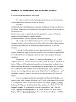
an example, Fig. 11.1 presents experimental results obtained by A. Aspect
and his collaborators in 1982. It gives the variation of E(α, β) as a function
of the difference α −β, which is found to be the only experimentally relevant
1
The precision has now been greatly improved with the use of photon pairs
produced by nonlinear splitting of ultraviolet photons (for a review, see e.g.
A. Aspect, Nature, vol. 398, p. 189 (18 March 1999)).
102 11 The EPR Problem and Bell’s Inequality
quantity.
Which theory, quantum mechanics or the simple hidden variable model de-
veloped above, gives a good account of the experimental data?
11.5 Bell’s Theorem and Experimental Results
As proved by Bell in 1965, the disagreement between the predictions of quan-
tum mechanics and those of hidden variable theories is actually very general
when one considers correlation measurements on entangled states. We now
show that the correlation results for hidden variable theories are constrained
by what is known as Bell’s inequality, which, however, can be violated by
quantum mechanics in specific experimental configurations.
Consider a hidden variable theory, whose result consists in two functions
A(λ, u
α

)andB(λ, u
β
) giving respectively the results of the electron and pro-
ton spin measurements. Each of these two functions takes only the two values
¯h/2and−¯h/2. It depends on the value of the hidden variable λ for the con-
sidered electron–proton pair. The nature of this hidden variable need not be
further specified for the proof of Bell’s theorem. The result A of course de-
pends on the axis u
α
chosen for the measurement of the electron spin, but
it does not depend on the axis u
β
. Similarly B does not depend on u
α
.This
locality hypothesis is essential for the following discussion.
Fig. 11.1. Measured variation of E(α, β) as a function of α − β. The vertical bars
represent the experimental error bars
11.6 Solutions 103
11.5.1. Give the correlation coefficient E(α, β) for a hidden variable theory
in terms of the functions A and B and the (unknown) distribution law P (λ)
for the hidden variable λ.
11.5.2. Show that for any set u
α
, u

α
, u
β
, u


β
, one has
A(λ, u
α
) B(λ, u
β
)+A(λ, u
α
) B(λ, u

β
)
+ A(λ, u

α
) B(λ, u

β
) − A(λ, u

α
) B(λ, u
β
)=±
¯h
2
2
. (11.4)
11.5.3. We define the quantity S as

S = E(α, β)+E(α, β

)+E(α

,β

) − E(α

,β) .
Derive Bell’s inequality
|S|≤2 .
11.5.4. Consider the particular case α − β = β

− α = α

− β

= π/4, and
compare the predictions of quantum mechanics with the constraint imposed
by Bell’s inequality.
11.5.5. The experimental results obtained by A. Aspect et al. are E(α, β)=
−0.66 (±0.04) for α−β = π/4andE(α, β)=+0.68 (±0.03) for α−β =3π/4.
Is a description of these experimental results by a local hidden variable theory
possible?
Are these results compatible with quantum mechanics?
11.6 Solutions
Section 11.1: The Electron Spin
11.1.1. In the eigenbasis |e : ± of
ˆ
S

ez
, the matrix of
ˆ
S
eϕ
is
¯h
2

cos ϕ sin ϕ
sin ϕ −cos ϕ

.
The eigenvalues of this operator are +¯h/2and−¯h/2.
11.1.2. The corresponding eigenvectors are
|e :+ϕ =cos
ϕ
2
|e :+ +sin
ϕ
2
|e : −
|e : − ϕ = −sin
ϕ
2
|e :+ +cos
ϕ
2
|e : −.
11.1.3. The probability amplitude is e :+α|e :+ϕ =cos((ϕ − α)/2) and

the probability P
+
(α)=cos
2
((ϕ −α)/2). Similarly P
−
(α)=sin
2
((ϕ −α)/2),
and the expectation value is, finally,

ˆ
S
eα
 =
¯h
2
cos (ϕ − α) .
104 11 The EPR Problem and Bell’s Inequality
Section 11.2: Correlations Between the Two Spins
11.2.1. The projector on the eigenstate |e :+α, corresponding to the mea-
sured value, is |e :+αe :+α|⊗
ˆ
I
p
,where
ˆ
I
p
is the identity operator on

the proton states. Therefore
P
+
(α)=|e :+α|e :+ϕ|
2
=cos
2
ϕ − α
2
,
and the state after measurement is |e :+α⊗|p : − ϕ. The proton spin
is not affected, because the initial state is factorized (all probability laws are
factorized).
11.2.2. One has 
ˆ
S
eα
 =
¯h
2
cos (ϕ − α)and
ˆ
S
pβ
 = −
¯h
2
cos (ϕ − β).
11.2.3. By definition, one has:
ˆ

S
2
eα
=
¯h
2
4
ˆ
I
e
and
ˆ
S
2
pβ
=
¯h
2
4
ˆ
I
p
and

ˆ
S
eα
⊗
ˆ
S

pβ
 = e :+ϕ|
ˆ
S
eα
|e :+ϕp : − ϕ|
ˆ
S
pβ
|p : − ϕ
= −
¯h
2
4
cos(ϕ − α)cos(ϕ −β) .
Therefore E(α, β) = 0. This just reflects the fact that in a factorized state,
the two spin variables are independent.
Section 11.3: Correlations in the Singlet State
11.3.1. There are two possible values:
¯h/2, corresponding to the projector |e :+αe :+α|⊗
ˆ
I
p
,and
−¯h/2, corresponding to the projector |e : − αe : − α|⊗
ˆ
I
p
.
Therefore, the probabilities are

P
+
(α)=
1
2

|e :+α|e :+|
2
+ |e :+α|e : −|
2

=1/2
and similarly P
−
(α)=1/2. This result is a consequence of the rotational
invariance of the singlet state.
11.3.2. The state after the measurement of the electron spin, yielding the
result +¯h/2, is
cos
α
2
|e :+α⊗|p : − − sin
α
2
|e :+α⊗|p :+ = |e :+α⊗|p :−α.
This simple result is also a consequence of the rotational invariance of the
singlet state, which can be written as
11.6 Solutions 105
|Ψ
s

 =
1
√
2
(|e :+α⊗|p : − α−|e : − α⊗|p :+α) .
Now the two possible results for the measurement of the proton spin ±¯h/2
have probabilities
P
+
(β)=sin
2
α − β
2
P
−
(β)=cos
2
α − β
2
.
11.3.3. If one had measured
ˆ
S
pβ
first, one would have found P
+
(β)=
P
−
(β)=1/2.

The fact that a measurement on the electron affects the probabilities for the
results of a measurement on the proton, although the two particles are spa-
tially separated, is in contradiction with Einstein’s assertion, or belief. This
is the starting point of the Einstein–Podolsky–Rosen paradox. Quantum me-
chanics is not a local theory as far as measurement is concerned.
Note, however, that this non-locality does not allow the instantaneous
transmission of information. From a single measurement of the proton spin,
one cannot determine whether the electron spin has been previously measured.
It is only when, for a series of experiments, the results of the measurements
on the electron and the proton are later compared, that one can find this
non-local character of quantum mechanics.
11.3.4. Individually, the expectation values vanish, since one does not worry
about the other variable:

ˆ
S
eα
 = 
ˆ
S
pβ
 =0.
11.3.5. However, the spins are correlated and we have

ˆ
S
eα
⊗
ˆ
S

pβ
 =
¯h
2
4

sin
2
α − β
2
− cos
2
α − β
2

and therefore E(α, β)=−cos(α − β).
Section 11.4: A Simple Hidden Variable Model
11.4.1. Using the results of Sect. 2, we have:

ˆ
S
eα
 =
¯h
2

cos(ϕ − α)
dϕ
2π
=0

and similarly 
ˆ
S
pβ
 = 0. We also obtain

ˆ
S
eα
⊗
ˆ
S
pβ
 = −
¯h
2
4

cos(ϕ − α)cos(ϕ − β)
dϕ
2π
= −
¯h
2
8
cos(α − β) .
106 11 The EPR Problem and Bell’s Inequality
Therefore, in this simple hidden variable model,
E(α, β)=−
1

2
cos(α − β).
In such a model, one finds a non-vanishing correlation coefficient, which is
an interesting observation. Even more interesting is that this correlation is
smaller than the prediction of quantum mechanics by a factor 2.
11.4.2. The experimental points agree with the predictions of quantum me-
chanics, and undoubtedly disagree with the results of the particular hidden
variable model we have considered. We must however point out that the data
given in the text is not the actual measured data. The “true” results are shown
in Fig. 11.2, where the error bars correspond only to statistical errors. The
difference from theory (i.e. quantum mechanics) is due to systematic errors,
mainly the acceptance of the detectors.
Fig. 11.2. Actual experimental variation of E(α, β) as a function of α − β
Section 11.5: Bell’s Theorem and Experimental Results
11.5.1. In the framework of a hidden variable theory, the correlation coeffi-
cient is
E(α, β)=
4
¯h
2

P (λ) A(λ, u
α
) B(λ, u
β
)dλ,
where P (λ) is the (unknown) distribution law for the variable λ, with
P (λ) > 0 ∀λ and

P (λ)dλ =1.

11.6 Solutions 107
Note that we assume here that the hidden variable theory reproduces the
one-operator averages found for the singlet state:
S
eα
 =

P (λ) A(λ, u
α
)dλ =0 S
pβ
 =

P (λ) B(λ, u
β
)dλ =0.
If this was not the case, such a hidden variable theory should clearly be re-
jected since it would not reproduce a well established experimental result.
11.5.2. The quantity of interest can be written:
A(λ, u
α
)

B(λ, u
β
)+B(λ, u

β
)


+ A(λ, u

α
)

B(λ, u

β
) − B(λ, u
β
)

.
The two quantities B(λ, u
β
)andB(λ, u

β
) can take only the two values ±¯h/2.
Therefore one has either
B(λ, u
β
)+B(λ, u

β
)=±¯hB(λ, u
β
) − B(λ, u

β

)=0
or
B(λ, u
β
)+B(λ, u

β
)=0 B(λ, u
β
) − B(λ, u

β
)=±¯h,
hence the result, since |A(λ, u
α
)| = |A(λ, u

β
)| =¯h/2.
11.5.3. We multiply the result (11.4) by P (λ) and integrate over λ. Bell’s
inequality follows immediately.
11.5.4. The quantum mechanical result for S is
S
Q
= −cos(α −β) − cos(α −β

) − cos(α

− β


)+cos(α

− β) .
In general, if we set θ
1
= α −β, θ
2
= β

−α, θ
3
= α

−β

, we can look for the
extrema of
f(θ
1
,θ
2
,θ
3
)=cos(θ
1
+ θ
2
+ θ
3
) − (cos θ

1
+cosθ
2
+cosθ
3
) .
The extrema correspond to θ
1
= θ
2
= θ
3
and sin θ
1
=sin3θ
1
, whose solutions
between 0 and π are θ
1
=0,π/4, 3π/4,π .Defining the function g(θ
1
)=
−3cosθ
1
+cos3θ
1
we have: g(0) = −2, g(π/4) = −2
√
2, g(3π/4) = 2
√

2,
g(π)=2.
We have represented the variation of g(θ) in Fig. 11.3. The shaded areas
correspond to results which cannot be explained by hidden variable theories.
In particular, for α −β = β

−α = α

−β

= π/4, we get S
Q
= −2
√
2, which
clearly violates Bell’s inequality. This system constitutes therefore a test of
the predictions of quantum mechanics vs. any local hidden variable theory.
11.5.5. The numbers given in the text lead to |3E(π/4) − E(3π/4)| =
2.66 (±0.15) in excellent agreement with quantum mechanics (2
√
2) but in-
compatible with hidden variable theories.
As in the previous question, the actual measurements were in fact E(π/4) =
−0.62 (±0.04), E(3π/4) = 0.60 (±0.03), therefore |3E(π/4) − E(3π/4)| =