Wind Farm Impact in Power System and Alternatives to Improve the Integration Part 11 pptx

Dynamic Simulation of Power Systems with Grid Connected Windfarms
239
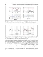
Fig. 19 and 20 show the response of the induction generator terminal voltage with
SVC/TCSC and STATCOM. /UPFC.
It can be concluded that terminal voltage of the DFIG is above 0.75 p.u. after 0.1 seconds.
Comparing Fig. 18, 19 and 20 it can be concluded that the UPFC improves the fault ride
through capability of the DFIG very effectively.





Fig. 19. Induction Generator Terminal Voltage – Effect of SVC and TCSC





Fig. 20. Induction Generator Terminal Voltage – Effect of STATCOM and UPFC
4.5 Effect of wind speed variations
The dynamic performance of the FACTS controllers with doubly fed induction generator
(DFIG) based wind farm is investigated using the wind speed model shown in Fig. 21.[7]
0.85
0.90
0.95
1.00
1.05
0123
4
5

Time (sec)
SVC
TCSC
Terminal
Voltage
(p.u)
0.92
0.94
0.96
0.98
1.00
1.02
0123
4
5
Time
(
sec
)
STATCOM
UPFC
Terminal
Voltage
(p.u)

Wind Farm – Impact in Power System and Alternatives to Improve the Integration
240

Fig. 21. Wind speed Model considered for long term dynamic simulation
The average wind speed is around 5 Km/h approximately. The wind speed data are
obtained by measuring the wind speed changes over an hour from the regional
meteorological website.
It can be observed that during the time period from 0- 1000 sec the wind speed fluctuates
around an average wind speed of 5 Km/h. But the wind speed reaches 16 Km/h around
1,200 seconds. The corresponding rotor speed variation by the induction generator is shown
in Fig 22. It can be observed that the rotor speed changes from its initial value to 1.25 p.u.
following wind speed increase at 1200 seconds.





Time (Sec)

Fig. 22. Rotor Speed response of DFIG
The corresponding active power variations are shown in Fig.23.
W
ind
Speed
(Km/h)
Rotor
Speed
(p.u.)

Dynamic Simulation of Power Systems with Grid Connected Windfarms
241

Time (Sec)
Fig. 23. Active Power Injected by the wind farm
The active power variations following the wind speed changes are highly fluctuating from
the steady state load flow level to the grid. The performance coefficient C
p
of the wind
turbine is kept as 0.48 in the algebraic equation
1
C.ρ.AV
2
3
p
P =
. Fig. 24 shows the impact of
an SVC/STATCOM controller on the rotor speed response of the DFIG.




Fig. 24. Rotor Speed Response of induction Generator with SVC/STATCOM
There are no significant rotor speed oscillations in the rotor speed of the induction generator
with SVC in the network; however the rotor speed increases to 1.26 p.u. with SVC in the
network following wind speed increase of 16 Km/h near 1200 seconds. The rotor speed
response of induction generator with TCSC/UPFC is shown in Fig 25.
0 200 400 600 800 1000 1200
1.08
1.10
1.12
1.14

1.16
1.18
1.20
1.22
1.24
1.26

Rotor
Speed

(p.u.)

Time(Sec)

SVC
STATCOM
Active
Power
Injected
M
W


Wind Farm – Impact in Power System and Alternatives to Improve the Integration
242
It can be noticed that the rotor speed oscillations are damped effectively with UPFC in the
network.


Fig. 25. Rotor speed Response of Induction generator with TCSC/UPFC.

5. Conclusion
For the simulation study the gains and time constants of the FACTS controllers are tuned
using a conventional optimization program, which minimizes the voltage /rotor speed
oscillations of the induction generator. Among series connected FACTS controllers the UPFC
damps both rotor angle oscillations of synchronous generators and rotor speed oscillations of
induction generator very effectively when compared with TCSC. This is due to the reactive
support provided by the shunt branch of the UPFC following the disturbance. However the
reactive power rating of UPFC is very high compared to that of the TCSC .It is suggested that a
STATCOM of suitable rating may be installed at the point of common coupling (PCC) with or
without a capacitor may be used for stabilizing rotor speed oscillations associated with doubly
fed variable speed induction generators following transient faults and disturbances.
The development of wind turbine and wind farm models is vital because as the level of
wind penetration increases it poses dynamic stability problems in the power system. For the

0200

400 600 800 1000 1200

1.09

1.10

1.11

1.12

1.13

1.14

1.15

1.16

1.17



Rotor
Speed

(p.u.)
Time(Sec)
TCSC
UPFC

Dynamic Simulation of Power Systems with Grid Connected Windfarms
243
present work we have taken a taken a doubly fed induction generator model and illustrated
the presence of sustained oscillations with wind farms. Suitable Flexible A.C.Transmission
Systems controllers are modeled using the non-linear simulation models and the transient
ratings of the FACTS controller are obtained to stabilize the rotor speed/rotor angle
oscillations in a DFIG based wind energy conversion scheme. The rotor speed stability of the
DFIG based system following a generator outage is studied. It can be observed that the
effect of low voltage ride through (LVRT) is very minimum following the contingency and
the presence of a FACTS device like the SVC improves the rotor speed stability.
This chapter also presented the results of a long term dynamic simulation of a grid
connected wind energy conversion system which simulated wind speed changes. From the
results it is observed that STATCOM and UPFC are effective candidates for damping the
rotor speed oscillations of the induction generator.

6. Appendix
a. Parameters
Base values for the per unit system conversion.
Base Power: 100 MVA, Base Voltage: 0.69 KV for low voltage bus bar, 150 KV for high
voltage busbar.
b. Doubly- Fed Induction Generator
Rated apparent power MVA: 2 MVA, Rotor inertia: 3.527 MW s/MVA
R
s
(p.u.) = 0.0693,X
s
(p.u.) = 0.080823,R
r
(p.u.) =0.00906,X
r
(p.u)= 0.09935,
X
m
(p.u) = 3.29, Minimum Rotor Speed: 0.56 p.u., Maximum Rotor Speed: 1.122 p.u.
c. Transformers
Three winding transformer (150 KV: 0. 69 KV), Primary rated apparent power=25 MVA,
Secondary rated apparent power = 25MVA,Tertiary rated apparent power = 6 MVA.
7. Acknowledgement
The author sincerely thanks Dr.M.Abdullah Khan, Professor of Eminence/EEE, B.S.Abdur
Rahman University (Formerly B.S.A.Crescent Engineering College) for his invaluable
guidance for completing the research work. The author sincerely thanks his father
Mr.
S.K.Natarajan & wife Mrs. Bhuvana for the moral support extended to him, at times of
pressure during the research work.
The author also wishes to place on record his sincere gratitude to

Mr.R.M.Kishore Vice
Chairman, RMK Engineering College and
Prof.Geetha Ramadas, Head of the Department,
Electrical and Electronics Engineering, RMK Engineering College, Tiruvallur District,
Tamilnadu, India.
8. References
Abdel – Magid Y.L. and El-Amin I.M., (1987)“Dynamic Stability of wind –turbine generators
under widely varying load conditions”,
Electrical Power and Energy Systems, Vol.9,
No.3, pp.180-188,1987.
Chai Chompoo-inwai, Wei-Jen Lee, Pradit Fuangfoo, Mitch Williams and James. R.Liao,
(2005), “System Impact study for the interconnection of wind generation and utility
system”,
IEEE Transactions on Industry Applications, Vol.41, No.1, pp.163- 168

Wind Farm – Impact in Power System and Alternatives to Improve the Integration
244
Claudio A. Canizares, Massimo Pozzi, Sandro Corsi, Edvina Uzunovic,(2003), “STATCOM
modelling for voltage and angle stability studies”,
Electrical Power and Energy
Systems
, Vol.25,pp.431-441.
Clemens Jauch, Poul Sorensen, Ian Norheim, Carsten Rasmussen, (2007) “Simulation of the
Impact of Wind power on the transient fault behavior of the Nordic Power
System”,
Electric Power System Research, Vol. 77, pp.135-144.
Haizea Gaztanaga, Ion Etxeberria-Ottadui, Dan Ocnasu,(2007) “Real time analysis of the
transient response improvement of wind farms by using a reduced scale
STATCOM prototype”,
IEEE Transactions on power systems, Vol.22, No.2, pp.658-

666.
-online website for wind speed data.
Istvan Erlich, Jorg Kretschmann, Jens Fortmann, Stephan Mueller-Engelhardt and Holger
Wrede, (2007),“Modeling of Wind Turbines Based on Doubly-Fed Induction
Generators for Power System Stability Studies”,
IEEE Transactions on Power Systems,
Vol.22, No.3, 2007, pp.909-919, 2007.
Kundur.P,(1994), “
Power System Stability and Control”, McGraw hill.
Lie Xiu, Yi Wang,(2007), “Dynamic Modeling and Control of DFIG based Wind Turbines
under Unbalanced Network Conditions
, IEEE Transactions on Power Systems, Vol.22,
No.1, pp. 314-323
Mohamed S.Elmoursi, Adel M.Sharaf,(2006), “Novel STATCOM controllers for voltage
stabilization of standalone Hybrid schemes”,
International Journal of Emerging
Electric Power Systems, Vol.7, Issue 3, Art 5,pp. 1-27.
Mohan Mathur R, Rajiv .K Varma, (2002),
Thyristor – Based FACTS controllers for electrical
transmission systems
, IEEE press, Wiley and Sons Publications
Nadarajah Mithulananthan, Claudio A. Canizares, Graham J.Rogers ,(2003), “Comparison of
PSS, SVC and STATCOM controllers for Damping Power System Oscillations”,

IEEE Transactions on Power Systems, Vol.8, No.2, pp.786-792.
Olof Samuelsson and Sture Lindahl, (2005),“On Speed Stability”,
IEEE Transactions on Power
Systems, Vol.20, No.2,pp. 1179-1180.
Senthil Kumar.N. , Abdullah Khan.M., (2008) ,“Impact of FACTS controllers on the dynamic
stability of power systems connected with Wind Farms”,

Wind Engineering, Vol.32,
No.2, pp.115-132.
Varma R.K. and Tejbir S.Sidhu, (2006)“Bibliographic Review of FACTS and HVDC
applications in Wind Power Systems”, International Journal of Emerging Electric
Power Systems, Vol.7, No. 3, pp. 1-16
Vladislav Akhmatov, (2003),“Analysis of dynamic behavior of electric power systems with
large amount of wind power”, Ph.D thesis, Technical University of Denmark
Dr.N.SENTHIL KUMAR is presently working as Professor in the department of Electrical
and Electronics Engineering, RMK Engineering College, Chennai. His area of
research includes modeling of FACTS devices for power system studies, modeling
of wind energy conversion systems for power system stability analysis.
Email:
Part 3
Modelling and Simulation
of Wind Power System

11
Modeling Wind Speed for
Power System Applications
Noha Abdel-Karim, Marija Ilic and Mitch J. Small
Carnegie Mellon University
USA
1. Introduction
The intermittent nature of wind power presents special challenges for utility system
operators when performing system economic dispatch, unit commitment, and deciding on
system energy reserve capacity. Also, participation of wind power in future electricity
markets requires more systematic modeling of wind power. It is expected that the installed
energy capacities from wind sources in the United States will increase by up to 20% by the
year 2020. New York Independent System Operator (NYISO), General Electric (GE), and
Automatic Weather Stations Inc., (AWS) conducted a project for the future of wind energy

integration in the United States. They stated that NY State has 101 potential wind energy
sites and it should be able to integrate wind generation up to at least 10% of system peak
load without further expansion (GE report 2005). In order to integrate wind power
systematically, it is necessary to solve the technical challenges as well as policy regulation
designs. Some of these polices have been updated to allow increased intermittent renewable
energy by settling imbalances in generation rulemakings and portfolio standards, where the
most commonly used one at this time is the production tax credit portfolios.
Due to intermittent nature of wind power, forecasting methods become a powerful tool and
of great importance to many power system applications that include uncertainties in
generation outputs. The recent work has discussed several methods to develop wind power
forecasting algorithms to anticipate the degrees of uncertainty and variability of wind
generation. (C. Lindsay & Judith, 2008) use an auto-regressive moving average model to
estimate the next ten-minute ahead production level for a hypothetical wind farm and
investigate the possibility of pairing wind output with responsive demand to reduce the
variability in the net wind output. In (Kittipong M. et al., 2007), the authors develop an
Artificial Neural Network (ANN) model to forecast wind generation power with 10-min
resolution. Current and previous wind speed and wind power generation are used as input
parameters to the network where the output from the ANN is the wind generation power.
(M. S. Miranda & R. W. Dunn, 2006) predicted one-hour-ahead of wind speed using both an
auto-regressive model and Bayesian approach. (D. Hawkins & M. Rothleder, 2006), discuss
operational concerns with increased amount of wind energy in the Day-ahead- and Hour-
ahead-Market for CAISO in California. They emphasize the importance of forecasting
accuracy for unit commitment and ancillary services and the implications of load following
or supplemental energy dispatch to rebalance the system every five minutes. In (Alberto F.
at el., 2005), the authors propose a probabilistic method to estimate the forecasting error for

Wind Farm – Impact in Power System and Alternatives to Improve the Integration

248
a Spanish Electricity System. They propose cost assessment with wind energy prediction

error. The assessment is developed to estimate the cost associated with any energy deviation
they cause. (Dale L. Osborn, 2006) discusses the impact of wind on the LMP market for
Midwest MISO at different wind penetrations level. His LMP calculations decrease with the
increase of wind energy penetration for the Midwest area. The authors of (Cameron W.
Potter at el., 2005) describe very short-term wind prediction for power generation, utilizing a
case study from Tasmania, Australia. They introduce an Adaptive Neural Fuzzy Inference
System (ANFIS) for short-term forecasting of a wind time series in vector form that contains
both wind speed and wind direction.
We next describe our modeling approach to derive a family wind models ranging from
short through and long term models. Using the same data, we illustrate achievable accuracy
of this model. This chapter presents three major parts in sections 2, 3 and 4. First, section 2
presents a short term wind speed linear prediction model in state space representation using
linear predictive coding (LPC), FIR and IRR filters. 10-minute, one-hour, 12-hour, and 24-
hour wind speed predictions are evaluated in least square error sense and the prediction
coefficients are then used in the state space stochastic formula representing past and future
predicted values. One year wind speed data in 10 minute resolution are first fitted by two
Weibull distribution parameters and then transformation to normal distribution is done for
prediction calculation purposes.
Second, section 3 of the chapter models wind speed patterns by decomposing it in different
time scales / frequency bands using the Fourier Transform. The decomposition ranges from
hourly (high frequency) up to yearly (low frequency), and are important in many power
grid applications. Short, medium and long-term wind speed trends require data analysis
that deals with changing frequencies of each pattern. By applying Fourier analysis to wind
speed signal, we aim to decompose it into three components of different frequencies, 1) Low
Frequency range: for economic development such as long term policies adaptation and
generation investment (time horizon: many years), 2) Medium Frequency range: for
seasonal weather variations and annual generation maintenance (time horizon: weeks but
not beyond a year), 3) High frequency range: for Intra-day and Intra-week variations for
regular generation dispatches and generation forced outage (time horizon: hours but within
a week). Each decomposed signal is presented in a lognormal distribution model and a

Discrete Markov process and the aggregated complete wind speed signal is also applied.
Third, section 4 presents the prediction results using past histories of wind data, which
support validity of Markov model. These independencies have been modeled as linear state
space discrete Markov process. A uniform quantization process is carried to discretize the
wind speed data using an optimum quantization step between different state levels for both
wind speed distributions used. Also state and transition probability matrices are evaluated
from the actual representation of wind speed data. Transition probabilities show smooth
transitions between consecutive states manifested by the clustering of transition
probabilities around the matrix diagonal.
2. Wind speed prediction model
2.1 Wind data distribution models
This prediction model uses more than 50 thousands samples of one-year wind speed data in
10-minute resolution. The data are used to determine the best fitted parameters of the

Modeling Wind Speed for Power System Applications

249
Weibull distribution model. Wind speed data are obtained from National weather station in
NYISO zonal areas by approximate longitudes and latitudes station’s allocation (National
weather station, Available online). The empirical cumulative distribution function (CDF) for
the wind speed random variable (RV) X has been evaluated using n samples based on the
statistical Weibull formula as (Noha Abdel-Karim at el., 2009):

()
ˆ
()
1
X
Rank x
Fx

n


(1)



Slope


Standard Error
(intercept)
Standard
error
(slope)
R-
square
0.0356 1.77
3
1.4 10


4
810


99.4%
Table I. Linear regression defines Weibull distribution parameters
Where a random variable X (R.V) represents wind speed, and “n” is the total sample size.
Knowing ahead that the wind speed RV is best characterized by the Weibull distribution

model:


1
1
()
x
X
x
a
fx x e
x
e
aa

















(2)


() 1
1
x
X
x
a
Fx e
e







(3)
Where in equation (2) or (3), we mention two alternate, yet equivalent forms of Weibull PDF
and CDF related by

1
a



 . Linear regression is performed between
ln( )Xx
, where x

is the data plotted on the horizontal axis, versus the following CDF metric on the vertical
axis:



ˆ
ln ln(1 ( ))
X
YFx  (4)
It is known that the PDF parameters are related to the linear regression slope m and Y-
intercept C, as follows:


exp( ) exp
slope m
Ca C





(5)
The regression results are shown in table I and both empirical and Weibull cumulative
distributions are plotted in figure 1.
Figure 1 presents a best Weibull distribution fit with the empirical CDF to wind speed data.
The next step is the transformation to normal distribution with mean zero and variance one.

Wind Farm – Impact in Power System and Alternatives to Improve the Integration

250

This transformation is used in both the fitting and prediction processes. The histograms of
wind speed signals in both Weibull and Normal distributions are shown in Figures 2 and 3,
respectively. By looking to Figure 3, the shape of the actual signal is shifted down with the
exact pattern due to the normalization process, (Noha Abdel-Karim at el., 2009).



0 2 4 6 8 10 12 14
0
0.1
0.2
0.3
0.4
0.5
0.6
0.7
0.8
0.9
1
Wind speed m/s
Cumulative Distribution Function
Empirical Lower bound Upper bound Weibull


Fig. 1. Empirical and Weibull Cumulative Distribution Functions.


-5 0 5 10 15 20 25
0
500

1000
1500
2000
2500
3000
3500
4000
4500
5000
Wind speed m/s
Frequency of occurence
Actual
Normalized


Fig. 2. Actual & normalized frequency occurrence of wind speed data.

Modeling Wind Speed for Power System Applications

251
Sep Oct Nov Dec Jan Feb March April May June July Aug Sep
-5
0
5
10
15
20
25
30
Tim e

Wind speed m/s
Actual Normalized

Fig. 3. Actual and normalized wind speed data.
2.2 Normalization of wind speed data
The initial step in the prediction process is data normalization. This step is done by
transforming the actual wind speed data X into Normal wind speed data, Xn (i.e., Xn is a
normalized Gaussian RV with zero mean and unit variance). This transformation is
performed using the Normal CDF inversion as follows:


1
() 1
()
() (0,1)
n
n
x
X
nXX
Xn
Fx e
xFFx
Fx G













(6)
Normal transformation is performed for the sole purpose of prediction, for both the fitting
and prediction processes. Figures 2 and 3 show the histograms and time series, respectively,
for both the actual (Weibull) wind speed X and Normal wind speed Xn. The shape of the
Normal signal Xn is shifted down with negative values (Figure 3) compared to the actual
signal X due to the normalization process.
2.3 Linear prediction and filter design
This section presents finite impulse response (FIR) and infinite impulse response (IRR)
filters. Both filters are being used to determine the prediction coefficients needed to process
the normalized wind speed signal x
n
, except that we drop the subscript “n” so as not to be
confused with the discrete time index. In discrete time, the Z-transform of a signal has been
used of a filter as follows:

() ( )  () 
i
ii
ii
gn g n i Gz gz






(General signal/IIR filter)

0
() ( 1)  ()
NN
i
ii
ii
hn h n Hz hz





(FIR filter)

Wind Farm – Impact in Power System and Alternatives to Improve the Integration

252
Where δ(n) is the Kronecker delta function. The wind speed random process x(n) is
characterized as wide sense stationary (WSS) Gaussian (Normal) process, and hence will
remain Gaussian after any stage of linear filtering. However, the wind speed process is NOT
white but can be closely modeled as Auto-Regressive (AR) process as will be shown next.
2.4 Linear Predictive Coding (LPC) and Finite Impulse Response Filter (FIR)
For prediction purposes of normalized wind speed data, we use Linear Predictive Coding
(LPC) based on the autocorrelation method to determine the coefficients of a forward linear
predictor. Prediction coefficients are calculated by minimizing the prediction error in the
least squares sense (P. P. Vaidyanathan, 2008). The method provides the LPC predictor and
its prediction error as follows:

1
1
ˆ
() ( )
ˆ
() () () () ( )
N
LPC i
i
N
NLPC i
i
xn bxni
en xn x n xn bxni


 

 


(7)
Where N is defined as the prediction order (using N past data samples) and the coefficients
{b1, , bN} are the fitting coefficients which minimize the mean square (MS) prediction error
signal. Yule-Walker (or normal) equations based on autocorrelation matrix have been used
to compute those prediction coefficients (P. P. Vaidyanathan, 2008). The LPC predictor has a
direct equivalent implementation as an FIR filter if we observe that the error Z-transform is
obtained as:

-1
N
1
E () X() B () X() B () E ()
B() 1
NN N
N
i
Ni
i
zz z z z z
zbz


   


(8)
Where BN(z) is the FIR filter transfer function used to compute the output error signal. In
other terms, it is also called the prediction polynomial (P. P. Vaidyanathan, 2008). Figure 4
shows how to obtain the output error signal using two equivalent forms: a) LPC prediction
and subtraction, and, b) direct FIR filter design, (Noha Abdel-Karim at el., 2009).


i
N
i
i
zb





1
)(X
ˆ
z
LPC
)(X z
)(E z
N
+
–


i
N
i
i
zb




1
1
)(E z
N
)(X z

(a) (b)
Fig. 4. Output prediction error signal using: a) LPC prediction and subtraction. b) Direct FIR
filter design.
To predict the normalized wind speed data, a forward LPC predictor
ˆ
()
LPC
xn can certainly
be used, but its accuracy is rather poor. However, the main advantage of LPC is that, as the
prediction order N increases sufficiently, the prediction error e
N
(n) tends to be closely
approximated as white noise (P. P. Vaidyanathan, 2008). This helps in modeling the Normal

Modeling Wind Speed for Power System Applications

253
wind speed as AR signal as will be shown next. Thus, forward LPC is considered an
important initial pre-coding step, (Noha Abdel-Karim at el., 2009).
2.5 Auto-Regressive (AR) model prediction and Infinite Impulse Response Filter (IIR)
filtering
The true wind speed can be obtained by multiplying the error signal E
N
(z) – if it is known –
by the inverse of the FIR filter
-1
N
B()z
, (Equation 8), which is now an all-pole IIR filter. If the
error signal is equivalent to white noise for large prediction order N, then the z-

multiplication (i.e., convolution or filtering in discrete time) now yields a signal that is
modeled as Gaussian Auto-Regressive (AR) process. Figure 5 shows the AR model block
diagram, while the reproduced AR signal is obtained by rewriting equation (7) in terms of
error as:

,
1
() ( ) ()
N
iN N
i
xn b xn i e n

  

(9)




i
N
i
i
zb




1

)(
ˆ
nx
LPC
)(nx
)(ne
N
+
–




N
i
i
i
zb
1
1
1
)(nx

Fig. 5. Auto-regression generation process using LPC estimation method
Equation (9) seems to be an ideal reproduction of
x(n) by inversion and it assumes the
following:
1.
The error signal is exactly updated in real time at the prediction time “n”. This is a genie
assisted

condition, as
ˆ
()
xn is not available yet!
2.
All the true N past data samples are available or exactly estimated (measured) by the
wind turbine speed meter and reported on time to the prediction algorithm.
3.
The prediction coefficients {b
1
, …, b
N
} are computed using the true past data samples
and updated for each new prediction.
In a practical prediction algorithm, these genie conditions do not hold. As for the prediction
error, different computation models can be used such as:
1.
Prediction error is estimated as a random generation of white noise of zero mean & unit
variance (P. P. Vaidyanathan, 2008).
2.
For initial or limited time intervals, the error can be exactly computed using true available
data samples to investigate the tracking of the algorithm, but not for long term
prediction.
3.
The prediction error can be estimated from exact measurements but up to a delay of one
or more samples, i.e., measurement at time (
n – L) applies at time “n”. For example, if
the prediction update interval is 10 minutes and the measurement delay is 1 hour, then
the sample count delay is
L = 60/10 = 6 samples. The minimum estimation delay is

L = 1.
In our work we excluded the white noise generation alternative and considered the two
other alternatives for wind speed forecasting.

Wind Farm – Impact in Power System and Alternatives to Improve the Integration

254
2.6 The prediction algorithm for wind speed
2.6.1 Linear prediction phases
More than 50,000 data samples collected in a 10-minute intervals have been used in this
short term prediction. A time reference
n = N
S
has been used which sets the end of known
data and start of prediction, where
N
S
≤ 50,000 and the remaining samples can be used for
tracking the algorithm.
A measurement reporting interval of
L samples has been assumed and that there is no error
in the measurement or the reporting process. At time epochs
n = N
S
+ m L , where m is
integer, the
L measurements x(n – L + 1), x(n – L + 2), …, x(n) are reported and will be
available to use at the next epoch, (
N
S

+ m L + 1). Depending on L, we have the following
extreme cases:
L = 1: → Point estimator case.
L = ∞: → Time series case, i.e., no estimation at all.
The following signals and associated time epochs have been defined for prediction purposes
as follows:
()xn : True Normal signal known within 0 ≤ n ≤ N
S
or whenever measurement is available as
above.
ˆ
()
xn : Predicted signal using IIR filter or AR recursion.
()
REF
xn: Reference signal used to produce
ˆ
()
xn .
()
REF
xn = ()xn within 0 ≤ n ≤ N
S
or whenever measurement is available
ˆ
() () ()
N
e n xn xn: True prediction error, only known if ()xn &
ˆ
()

xn are known.
ˆ
()
N
en: Prediction error estimate, either white noise or delayed measurement.
The prediction algorithm can be summarized as follows:
a. Training phase within 0 ≤ n ≤ N
S
: Apply the LPC algorithm on the true samples x(0), … ,
x(N
S
) to obtain the prediction coefficients {1, b
1
, …, b
N
}. Then we filter the same samples
using the FIR coefficients {–b
1
, …, –b
N
} to compute the predictor
ˆ
()
xn and true
prediction error
ˆ
() () ()
N
e n xn xn


 within 0 ≤ n ≤ N
S
. Further, we pre-load the reference
signal ()
REF
xn = ()xn within 0 ≤ n ≤ N
S
.
Prediction phase for n ≥ N
S
+ 1: We apply the AR model of equation (9) after computing the
error estimate
ˆ
()
N
en. We use the same prediction coefficients obtained in the training phase
if we plan short-term prediction, which is our case. Otherwise, we have to update the
coefficients for long-term prediction. The steps for prediction at epoch “
n” are given by:
1.
Compute the prediction error estimate using:

ˆˆ
() ( 1) ( 1)if ( 1) ( 1)
ˆˆ ˆ
(2)(1),if (1)(1)
NREF REF
REF
e n x n xn x n xn
xn xn x n xn


   

   
(10)
We can set
ˆ
()
N
en as randomly generated white noise or also import a snapshot from
the past true prediction error series obtained in the training phase.
2.
By inspecting equation (9), we compute the predicted signal via the AR recursion:

,
1
ˆˆ
() ( ) ()
N
AR i N REF N
i
xn bx nien

  

(11)

Modeling Wind Speed for Power System Applications

255

3. Update the reference signal entries as follows:
If n ≠ N
S
+ m L →
ˆ
() ()
REF AR
xnxn


If n = N
S
+ m L → b [x
REF
(n – L + 1),
x
REF
(n – L + 2), …, x
REF
(n)] = [x(n – L + 1), x(n – L + 2), …, x(n)]
4.
Update the prediction coefficients if needed by running the LPC on the reference signal.
It is best to make such update at n = N
S
+ m L because x
REF
(n) would be just updated by
measurements.
5. Increment n and go back to step 1.
Figure 6 shows the two phases of the prediction process

n
0
N
S
N
S
+L
N
S
+2L
…
Training phase / LPC
AR prediction
Update
measurements
Known
data

Fig. 6. The two phases of prediction process.
2.6.2 Wind speed prediction results
Wind speed data have been gathered from Dunkirk weather station in the west zone of New
York State. Those data have been used for the stochastic prediction of wind speed (National
Weather Station, Available online).

0 4 8 12 16 20 24
-2
-1.5
-1
-0.5
0
0.5
1
1.5
2
Hour
N
orma
li
ze
d

Wi
n
d
spee
d

10 min 1 hour Actual

Fig. 7. Ten minutes and one hour prediction using 10 minute past value
Figures 7 and 8 assist remarkable observation that the prediction model insensitive to the
prediction order which is defined as the number of observed data (history) used in the

Wind Farm – Impact in Power System and Alternatives to Improve the Integration

256
prediction. The 10-minute wind speed prediction model shows persistence for all prediction
orders used.

0 2 4 6 8 10 12 14 16 18 20 22 24
-1.5
-1
-0.5
0
0.5
1
1.5
2
Hour
N
orma
li
ze
d

Wi
n
d
spee
d
10 min 1 hour Actual

Fig. 8. Ten min and one hour prediction using 1 hour past values
The effect of how the increase in the number of present and past wind speed sample data

does not significantly reduce the root mean square error (RMSE), (Figure 9). This led us to
an interesting valuation of data structuring and modeling. If only can one recent sample
random variable captures stochastic statistics of wind signal to predict future values, then
time and memory reductions in presenting such signal can be modeled as a discrete Markov
process; the process that stated generally the independencies between past and present
values to present signal statistics and structure using state and transition probabilities that
will be discussed in detail later.
3. Wind speed signal decomposition
In electricity markets, decisions of utility companies on power selling/buying, production
levels, power plants scheduling and investment are made with risks and uncertainties due
to volatility and unpredictability of renewable energy patterns. For that, coming up with
reasonable modeling of wind speed in different patterns with different time scales, ranging
from hours up to few years, are of most importance in many power grid applications. In
doing so, different wind signal trends require different data analyses that capture different
frequencies. Those frequencies are defined as:
1.
Low frequency range: for economic development such as long term policies adaptation
and generation investment, (time horizon: many years)
2. Medium frequency range: To detect seasonal weather variations, and therefore help in
assigning mid-term generation capacities which influence electricity market prices and
power grid generation planning for few weeks with no effect beyond a year.
3.
High frequency range: for Intra-day and Intra-week variations for regular generation
dispatches and forced generation outage, for fast variations of few hours but not
beyond a week.

Modeling Wind Speed for Power System Applications

257

Fig. 9. Wind speed prediction using various past wind speed data in 10 minute resolution:
1
st
raw: 10 minute prediction using: (a) 10 min, (b) one hour, (c) 12 hours, and (d) 24 hours
past data.
2
nd
raw: 1 hour prediction using: (e) 10 min. , (f) one hour, (g) 12 hours , and (h) 24 hours
past data.
3
rd
raw: 12 hours prediction using: (i) 10 min. , (j) one hour, (k) 12 hours , and (l) 24 hours
past data.
4
th
raw: 24 hours prediction using: (m) 10 min. , (n) one hour, (o) 12 hours , and (p) 24 hours
past data.
In this section, short, medium and long-terms wind speed trends have been decomposed by
applying Discrete Fourier transform (Yang HE, 2010).
A Discrete Fourier Transform (DFT) X[k], is computed for the natural logarithm of wind
speed signal, x[n]. The DFT is then decomposed in frequency domain into low, medium and
high frequency components, each of different frequency index range as:

Wind Farm – Impact in Power System and Alternatives to Improve the Integration

258
[] [] [] []
LMH

Xk X k X k X k

 (12)
Where X
L
[k], X
M
[k] and X
H
[k] are the low, medium and high frequency components,
respectively. The DFT applies only to finite discrete signal (i.e., sequence of length “N”).

10][



Nnfornx

Where n is a discrete time index. The DFT, X[k], is also a discrete sequence of length “N”
and k is a discrete frequency index. The main frequency coefficients for each component are
given by:

[] ,0
[]
0 ,/2
[] ,
[]
0,
[] , /2
[]

0,0
y
L
y
yd
M
d
H
d
Xk k k
Xk
kkN
Xk k k k
Xk
otherwise
Xk k k N
Xk
kk






















(13)
It is noted that the DFT X[k] exhibits complex conjugate symmetry around k = N/2; hence all
the decomposition components in (13) have conjugate symmetric coefficients within
/2 1NkN . The thresholds k
y
, k
w
and k
d
are the yearly, weekly and daily discrete
frequency indices and are related to their analog frequency values by:

8760
168
24
y
s
s
y
sws
w

sds
d
k
f
f
f
N
f
k
f
f
N
fkf
f
N



(14)
Where f
s
= 1 sample/hr is the sampling frequency and N is the sample size covering 16
years from 1994 till 2009 in hourly resolution (National Weather Station, Available online).
Then we take the Inverse DFT (IDFT) of each component in (13), we obtain the aggregated
IDFT of (12) in time domain:

[] [] [] []
tLMH
xn xn x n x n


 (15)

Each IDFT signal component in (15) is modeled as a Gaussian time series. By taking the
exponent of each signal in (15), we obtain the log-normal time domain signals that represent
the low, medium and high frequency components of the original wind speed signal. Each
pattern can be used to characterize the behavior of wind speed for different purposes.
Figure 10 shows the aggregation of the three log-normal wind speed components in the time
domain. Each decomposed wind speed signal is of important use in different applications in
power systems, e.g., wind power predictions, scheduling and investment decisions.

Modeling Wind Speed for Power System Applications

259



() () () ()
tHML
xt x t x t x t







Fig. 10. Construction of wind speed signal using low, medium and high frequency
components
I. x
H

(t)
II. x
M
(t)
III. x
L
(t)

Wind Farm – Impact in Power System and Alternatives to Improve the Integration

260
4. Discrete Markov process
The interesting results obtained in section 2 (Figure 9) show Independencies from past
observed data except for the nearest one. Model representation using Markov process is
then valid, which is defined as the likelihood of next wind speed value in state k is
conditioned on the most recent value of wind speed in state m. Equation (15) defines this
likelihood – state relationship.

11
(,,,)()
kmmm kmm
PX iX x x X
j
PX iX x

  
(15)
However, to identify state levels and state values, uniform midrise quantization process is
carried out to discretize wind speed signal to state levels with optimum threshold or cutoffs
values.

4.1 Design of optimum uniform quantizer
A midrise uniform Quantizer has been implemented that minimizes the mean square
quantization error given a set of M states; we define
12
[]
M
xxx x  as a state value vector,
and
[ (1) (2) ( 1)]
ttt t
xxx xM as a quantized threshold levels or partitions vector. x is the
original analog wind speed signal and
q
x is the quantization signal. The quantization step 
is defined as;

(1)()(1)()
tt
xm xm x m x m

   (16)
The uniform Quantizer works as follows:

(1) (1)
() ( 1)
() ( 1) ()
t
qt
tt
xifxx

xxMifxxM
xm ifx m x x m










(17)
4.2 State and transition probabilities in discrete state space Markov model
Given the initial and final boundaries of each state; state probabilities can now be defined as:


()
()
() () ()
() ()
(() (())
f
i
if
xm
X
xm
Xf Xi
Pm P x m x x m

Pxm
f
xdx
Fxm Fxm









(18)
Where m is defined as any given state index and has the range from m= 1 to m=M. Equation
(19) presents Markov linear state space model that takes prediction coefficients error signal
modeled as disturbance d, and a regeneration time

in which the signal updates itself, for
example updates every 10 minutes (1 sample), or every one hour (6 samples) and so on.

1
() ( ) ()
N
jj
j
xn axn j dn





(19)
we define a processing time from
o


 by a rectangular function. Equations (20) and (21)
define subsequent use of state space representation.

Modeling Wind Speed for Power System Applications

261

1
,1
1
() ( ) ()
N
jj j
j
xn axn
j
dn






(20)



,1,
() () ()
jjj
xn Ax ndn


  (21)

Where


A is the prediction coefficient matrix. Transition probabilities are calculated based
on the counting method discussed in [11], in which we define :
(| )
trans
Nkm The number of transitions from state m to state k in the time series,(m is the
originating state, k is the next state)
()
state
Nm The number of occurrences of state m in the time series signal.
Both state and transition counters are related by (22) and the total size of the time series is
defined in (23)

1
() (|)
M
state trans

k
Nm N km



(22)

111
() (|)
MMM
state trans
mmk
NNm Nkm



(23)
Using the statistical counter values of
()
state
Nmand (| )
trans
Nkm, the transition and state
probabilities can be statistically computed as:

(| )
(| )
()
trans
trans

state
Nkm
Pkm
Nm
 (24)

()
()
state
state
Nm
Pm
N

(25)
Where, K = 1,…, M and, m= 1,…, M. Note that (25) represent the statistical (actual) state
probabilities of wind speed signal while (18) represent the theoretical state probabilities
defined be either Weibull or Normal probability density functions. The probability state
space representation is defined as:



,1,
(()) ()
jtransj
Px n P x n


 (26)
Where



P is the transition probability matrix.
In Figures 11, transition probability plots of normalized wind speed data are shown. The
plots are generated from the same one-year sample size used in short term prediction
(section 2). Those transition probabilities obviously appeared in cluster around the diagonal.
This means smooth transitions between states and suggesting that the data does not exhibit
frequent wind gusts. Moreover, we see the difference between theoretical and actual
(statistical state probabilities (Figures 17 & 18). The reason is due to the use of the uniform
quantization while we conjecture that a non-uniform quantizer will achieve a better match
between the actual and theoretical probabilities.

Wind Farm – Impact in Power System and Alternatives to Improve the Integration

262
5
10
15
5
10
15
0
0.2
0.4
0.6
0.8
1
Ori
g
inal State

Next State
Transition Probability

Fig. 11. Gaussian transition probabilities for M = 16 states

5
10
15
5
10
15
0
0.2
0.4
0.6
0.8
1
Original State
Next State
Transition Probability

Fig. 12. Weibull transition probabilities for M = 16 states

Modeling Wind Speed for Power System Applications

263
5
10
15
20

25
30
10
20
30
0
0.2
0.4
0.6
0.8
1
Original State
Next State
Transition Probability

Fig. 13. Gaussian transition probabilities for M = 32 states
5
10
15
20
25
30
10
20
30
0
0.2
0.4
0.6
0.8

1
Original State
Next State
Transition Probability

Fig. 14. Weibull transition probabilities for M = 32 states