The Quantum Mechanics Solver 15 docx

14.6 Solutions 139
The vector |α is normalized:
α|α =e
−|α|
2
∞

n=0
(α
∗
)
n
α
n
n!
=1.
The expectation value of the number of photons in that state is:
n = α|
ˆ
N|α = α|ˆa
†
ˆa|α = ||ˆa|α||
2
= |α|
2
.
(b) The time evolution of |ψ(t) is given by
|ψ(t) =e
−|α|
2
/2

∞

n=0
α
n
√
n!
e
−iω(n+1/2)t
|n
=e
−iωt/2
e
−|α|
2
/2
∞

n=0

αe
−iωt

n
√
n!
|n
=e
−iωt/2
|(αe

−iωt
) .
(c) The expectation values of the electric and magnetic fields are
E(r)
t
=2α cos ωt sin kz

¯hω

0
V
u
x
B(r)
t
= −2α sin ωt cos kz

¯hωµ
0
V
u
y
.
(d) These fields are of the same type as the classical fields considered at the
beginning of the problem, with
e(t)=2α

¯hω

0

V
cos ωt b(t)=−2α

¯hωµ
0
V
sin ωt .
Given the relation 
0
µ
0
c
2
=1,weverifythat ˙e(t)=c
2
kb(t)and
˙
b = −ke(t).
Therefore the expectation values of the field operators satisfy Maxwell’s equa-
tions.
(e) The energy of the classical field can be calculated using the result of ques-
tion 1.1b. Since cos
2
ωt +sin
2
ωt = 1, we find U(t)=¯hωα
2
. This “classical”
energy is therefore time-independent. The expectation value of
ˆ

H
C
is:
H
C
 = ¯hω(N +1/2) =¯hω(α
2
+1/2) .
It is also time independent (Ehrenfest’s theorem).
(f) For |α| much larger than 1, the ratio U(t)/H
C
 is close to 1. More
generally, the expectation value of a physical quantity as calculated for a
quantum field in the state |α, will be close to the value calculated for a
classical field such that E
cl
(r,t)=E(r)
t
and B
cl
(r,t)=B(r)
t
.
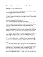
140 14 Direct Observation of Field Quantization
Fig. 14.4. (a) Positions of the five first energy levels of H
0
.(b) Positions of the five
first energy levels of
ˆ
H =

ˆ
H
0
+
ˆ
W
Section 14.2: The Coupling of the Field with an Atom
14.2.1. One checks that
ˆ
H
0
|f,n =

−
¯hω
A
2
+

n +
1
2

¯hω

|f,n ,
ˆ
H
0
|e, n =


¯hω
A
2
+

n +
1
2

¯hω

|e, n .
14.2.2. For a cavity which resonates at the atom’s frequency, i.e. if ω = ω
A
,
the couple of states |f,n+1, |e, n are degenerate. The first five levels of
ˆ
H
0
are shown in Fig. 14.4a. Only the ground state |f,0 of the atom+field system
is non-degenerate.
14.2.3. (a) The action of
ˆ
W on the basis vectors of H
0
is given by:
ˆ
W |f,n =
√

nγ|e, n −1 if n ≥ 1
=0 if n =0
ˆ
W |e, n =
√
n +1γ |f,n +1 .
The coupling under consideration corresponds to an electric dipole interaction
of the form −
ˆ
D ·
ˆ
E(r), where
ˆ
D is the observable electric dipole moment of
the atom.
(b)
ˆ
W couples the two states of each degenerate pair. The term ˆaˆσ
+
corre-
sponds to the absorption of a photon by the atom, which undergoes a transi-
tion from the ground state to the excited state. The term ˆa
†
ˆσ
−
corresponds
to the emission of a photon by the atom, which undergoes a transition from
the excited state to the ground state.
14.6 Solutions 141
14.2.4. The operator

ˆ
W is block-diagonal in the eigenbasis of
ˆ
H
0
{|f,n, |e, n}. Therefore:
• The state |f, 0 is an eigenstate of
ˆ
H
0
+
ˆ
W with the eigenvalue 0.
• In each eigen-subspace of
ˆ
H
0
generated by {|f,n +1, |e, n} with n ≥ 0,
one must diagonalize the 2 ×2 matrix:

(n +1)¯hω ¯hΩ
n
/2
¯hΩ
n
/2(n +1)¯hω

whose eigenvectors and corresponding eigenvalues are (n ≥ 0):
|φ
+

n
 corresponding to E
+
n
=(n +1)¯hω +
¯hΩ
n
2
|φ
−
n
 corresponding to E
−
n
=(n +1)¯hω −
¯hΩ
n
2
.
The first five energy levels of
ˆ
H
0
+
ˆ
W are shown in Fig. 14.4b.
Section 14.3: Interaction of the Atom and an “Empty” Cavity
14.3.1. We expand the initial state on on the eigenbasis of
ˆ
H:

|ψ(0) = |e, 0 =
1
√
2

|φ
+
0
−|φ
−
0


.
The time evolution of the state vector is therefore given by:
|ψ(t) =
1
√
2

e
−iE
+
0
t/¯h
|φ
+
0
−e
−iE

−
0
t/¯h
|φ
−
0


=
e
−iωt
√
2

e
−iΩ
0
t/2
|φ
+
0
−e
iΩ
0
t/2
|φ
−
0



.
14.3.2. In general, the probability of detecting the atom in the state f ,in-
dependently of the field state, is given by:
P
f
(T )=
∞

n=0
|f,n|ψ(T)|
2
.
In the particular case of an initially empty cavity, only the term n =1con-
tributes to the sum. Using |f,1 =

|φ
+
0
 + |φ
−
0


/
√
2, we find
P
f
(T )=sin
2

Ω
0
T
2
=
1
2
(1 −cos Ω
0
T ) .
It is indeed a periodic function of T , with angular frequency Ω
0
.
14.3.3. Experimentally, one measures an oscillation of frequency ν
0
= 47 kHz.
This result corresponds to the expected value:
ν
0
=
1
2π
2d
¯h

¯hω

0
V
.

142 14 Direct Observation of Field Quantization
Section 14.4: Interaction of an Atom with a Quasi-Classical State
14.4.1. Again, we expand the initial state on the eigenbasis of
ˆ
H
0
+
ˆ
W :
|ψ(0) = |e⊗|α =e
−|α|
2
/2
∞

n=0
α
n
√
n!
|e, n
=e
−|α|
2
/2
∞

n=0
α
n

√
n!
1
√
2

|φ
+
n
−|φ
−
n


.
At time t the state vector is
|ψ(t) =e
−|α|
2
/2
∞

n=0
α
n
√
n!
1
√
2


e
−iE
+
n
t/¯h
|φ
+
n
−e
−iE
−
n
t/¯h
|φ
−
n


.
We therefore observe that:
• the probability to find the atom in the state |f and the field in the state
|0 vanishes for all values of T ,
• the probability P
f
(T,n) can be obtained from the scalar product of |ψ(t)
and |f,n +1 =(|φ
+
n
 + |φ

−
n
) /
√
2:
P
f
(T,n)=
1
4
e
−|α|
2
|α|
2n
n!



e
−iE
+
n
t/¯h
− e
−iE
−
n
t/¯h




2
=e
−|α|
2
|α|
2n
n!
sin
2
Ω
n
T
2
=
1
2
e
−|α|
2
|α|
2n
n!
(1 −cos Ω
n
T ) .
14.4.2. The probability P
f
(T ) is simply the sum of all probabilities P

f
(T,n):
P
f
(T )=
∞

n=0
P
f
(T,n)=
1
2
−
e
−|α|
2
2
∞

n=0
|α|
2n
n!
cos Ω
n
T.
14.4.3. (a) The three most prominent peaks of J(ν) occur at the frequencies
ν
0

= 47 kHz (already found for an empty cavity), ν
1
= 65 kHz and ν
2
=
81 kHz.
(b) The ratios of the measured frequencies are very close to the theoretical
predictions: ν
1
/ν
0
=
√
2andν
2
/ν
0
=
√
3.
(c) The ratio J(ν
1
)/J(ν
0
) is of the order of 0.9. Assuming the peaks have
the same widths, and that these widths are small compared to the splitting
ν
1
− ν
0

, this ratio correponds to the average number of photons |α|
2
in the
cavity.
Actually, the peaks overlap, which makes this determination somewhat
inaccurate. If one performs a more sophisticated analysis, taking into account
the widths of the peaks, one obtains |α|
2
=0.85 ± 0.04 (see the reference at
end of this chapter).
Comment: One can also determine |α|
2
from the ratio J(ν
2
)/J(ν
1
)which
should be equal to |α|
2
/2. However, the inaccuracy due to the overlap of the
peaks is greater than for J(ν
1
)/J(ν
0
), owing to the smallness of J(ν
2
).
14.6 Solutions 143
Section 14.5: Large Numbers of Photons: Damping and Revivals
14.5.1. The probability π(n) takes significant values only if (n −n

0
)
2
/(2n
0
)
is not much larger than 1, i.e. for integer values of n in a neighborhood of n
0
of relative extension of the order of 1/
√
n
0
.Forn
0
 1, the distribution π(n)
is therefore peaked around n
0
.
14.5.2. (a) Consider the result of question 4.2, where we replace Ω
n
by its
approximation (14.5):
P
f
(T )=
1
2
−
1
2

∞

n=0
π(n)cos

Ω
n
0
+ Ω
0
n −n
0
2
√
n
0
+1

T

(14.6)
We now replace the discrete sum by an integral:
P
f
(T )=
1
2
−
1
2


∞
−∞
e
−u
2
/(2n
0
)
√
2πn
0
· cos

Ω
n
0
+ Ω
0
u
2
√
n
0
+1

T

du.
We have extended the lower integration bound from −n

0
down to −∞,using
the fact that the width of the gaussian is
√
n
0
 n
0
. We now develop the
expression to be integrated upon:
cos

Ω
n
0
+Ω
0
u
2
√
n
0
+1

T

= cos (Ω
n
0
T )cos


Ω
0
uT
2
√
n
0
+1

− sin (Ω
n
0
T )sin

Ω
0
uT
2
√
n
0
+1

.
The sine term does not contribute to the integral (odd function) and we find:
P
f
(T )=
1

2
−
1
2
cos (Ω
n
0
T )exp

−
Ω
2
0
T
2
n
0
8(n
0
+1)

.
For n
0
 1, the argument of the exponential simplifies, and we obtain:
P
f
(T )=
1
2

−
1
2
cos (Ω
n
0
T )exp

−
T
2
T
2
D

with T
D
=2
√
2/Ω
0
.
(b) In this approximation, the oscillations are damped out in a time T
D
which
is independent of the number of photons n
0
. For a given atomic transition
(for fixed values of d and ω), this time T
D

increases like the square root of
the volume of the cavity. In the limit of an infinite cavity, i.e. an atom in
empty space, this damping time becomes infinite: we recover the usual Rabi
oscillation. For a cavity of finite size, the number of visible oscillations of
P
f
(T ) is roughly ν
n
0
T
D
∼
√
n
0
.
144 14 Direct Observation of Field Quantization
(c) The function P
f
(T ) is made up of a large number of oscillating functions
with similar frequencies. Initially, these different functions are in phase, and
their sum P
f
(T ) exhibits marked oscillations. After a time T
D
, the various os-
cillations are no longer in phase with one another and the resulting oscillation
of P
f
(T ) is damped. One can find the damping time by simply estimating

the time for which the two frequencies at half width on either side of the
maximum of π(n)areoutofphasebyπ:
Ω
n
0
+
√
n
0
T
D
∼ Ω
n
0
−
√
n
0
T
D
+ π and

n
0
±
√
n
0

√

n
0
±
1
2
⇒ Ω
0
T
D
∼ π.
14.5.3. Within the approximation (14.5) suggested in the text, equation
(14.6) above corresponds to a periodic evolution of period
T
R
=
4π
Ω
0
√
n
0
+1.
Indeed

Ω
n
0
+ Ω
0
n −n

0
2
√
n
0
+1

T
R
=4π (n
0
+1)+2π(n −n
0
) .
We therefore expect that all the oscillating functions which contribute to
P
f
(T ) will reset in phase at times T
R
,2T
R
,. . . The time of the first revival,
measured in Fig. 14.3, is Ω
0
T  64, in excellent agreement with this predic-
tion. Notice that T
R
∼ 4
√
n

0
T
D
, which means that the revival time is always
large compared to the damping time.
Actually, one can see from the result of Fig. 14.3 that the functions are
only partly in phase. This comes from the fact that the numerical calculation
has been done with the exact expression of Ω
n
. In this case, the difference
between two consecutive frequencies Ω
n+1
− Ω
n
is not exactly a constant,
contrary to what happens in approximation (14.5); the function P
f
(T )isnot
really periodic. After a few revivals, one obtains a complicated behavior of
P
f
(T ), which can be analysed with the techniques developed for the study of
chaos.
14.7 Comments
The damping phenomenon which we have obtained above is “classical”: one
would obtain it within a classical description of the interaction of the field
and the atom, by considering a field whose intensity is not well defined (this
would be the analog of a distribution π(n) of the number of photons). On the
other hand, the revival comes from the fact that the set of frequencies Ω
n

is
discrete. It is a direct consequence of the quantization of the electromagnetic
14.7 Comments 145
field, in the same way as the occurrence of frequencies ν
0
√
2, ν
0
√
3, in the
evolution of P
f
(T ) (Sect. 4).
The experiments described in this chapter have been performed in Paris,
at the Laboratoire Kastler Brossel. The pair of levels (f,e) correspond to very
excited levels of rubidium, which explains the large value of the electric dipole
moment d. The field is confined in a superconducting niobium cavity (Q-
factor of ∼ 10
8
), cooled down to 0.8 K in order to avoid perturbations to the
experiment due to the thermal black body radiation (M. Brune, F. Schmidt-
Kaler, A. Maali, J. Dreyer, E. Hagley, J M. Raimond, and S. Haroche, Phys.
Rev. Lett. 76, 1800 (1996)).
15
Ideal Quantum Measurement
In 1940, John von Neumann proposed a definition for an optimal, or “ideal”
measurement of a quantum physical quantity. In this chapter, we study a
practical example of such a procedure. Our ambition is to measure the exci-
tation number of a harmonic oscillator S by coupling it to another oscillator
D whose phase is measured.

We recall that, for k integer:
N

n=0
e
2iπkn
N+1
= N + 1 for k = p(N +1),pinteger ; = 0 otherwise.
15.1 Preliminaries: a von Neumann Detector
We want to measure a physical quantity A on a quantum system S.Weuse
a detector D devised for such a measurement. There are two stages in the
measurement process. First, we let S and D interact. Then, after S and D
get separated and do not interact anymore, we read a result on the detector
D. We assume that D possesses an orthonormal set of states {|D
i
} with
D
i
|D
j
 = δ
i,j
. These states correspond for instance to the set of values
which can be read on a digital display.
Let |ψ be the state of the system S under consideration, and |D the state
of the detector D. Before the measurement, the state of the global system
S + D is
|Ψ
i
 = |ψ⊗|D .

Let a
i
and |φ
i
 be the eigenvalues and corresponding eigenstates of the
observable
ˆ
A. The state |ψ of the system S canbeexpandedas
|ψ =

i
α
i
|φ
i
 . (15.1)
148 15 Ideal Quantum Measurement
15.1.1. Using the axioms of quantum mechanics, what are the probabilities
p(a
i
) to find the values a
i
in a measurement of the quantity A on this state?
15.1.2. After the interaction of S and D, the state of the global system is in
general of the form
|Ψ
f
 =

i,j

γ
ij
|φ
i
⊗|D
j
 (15.2)
We now observe the state of the detector. What is the probability to find the
detector in the state |D
j
?
15.1.3. After this measurement, what is the state of the global system S+D?
15.1.4. A detector is called ideal if the choice of |D
0
 and of the coupling S–
D leads to coefficients γ
ij
which, for any state |ψ of S, verify: |γ
ij
| = δ
i,j
|α
j
|.
Justify this designation.
15.2 Phase States of the Harmonic Oscillator
We consider a harmonic oscillator of angular frequency ω. We note
ˆ
N the
“number” operator, i.e. the Hamiltonian is

ˆ
H =(
ˆ
N +1/2))¯hω with eigen-
states |N and eigenvalues E
N
=(N +
1
2
)¯hω, N integer ≥ 0.
Let s be a positive integer. The so-called “phase states” are the family of
states defined at each time t by:
|θ
m
 =
1
√
s +1
N=s

N=0
e
−iN(ωt+θ
m
)
|N (15.3)
where θ
m
can take any of the 2s +1values
θ

m
=
2πm
s +1
(m =0, 1, ,s) . (15.4)
15.2.1. Show that the states |θ
m
 are orthonormal.
15.2.2. We consider the subspace of states of the harmonic oscillator such
that the number of quanta N is bounded from above by some value s.The
sets {|N ,N =0, 1, ,s} and {|θ
m
,m =0, 1, ,s} are two bases in this
subspace. Express the vectors |N in the basis of the phase states.
15.2.3. What is the probability to find N quanta in a phase state |θ
m
?
15.2.4. Calculate the expectation value of the position ˆx in a phase state,
and find a justification for the name “phase state”. We recall the relation
ˆx|N = x
0
(
√
N +1|N +1 +
√
N |N − 1), where x
0
is the characteristic
length of the problem. We set C
s

=

s
N=0
√
N.
15.4 An “Ideal” Measurement 149
15.3 The Interaction between the System
and the Detector
We want to perform an “ideal” measurement of the number of excitation
quanta of a harmonic oscillator. In order to do so, we couple this oscillator
S with another oscillator D, which is our detector. Both oscillators have the
same angular frequency ω. The eigenstates of
ˆ
H
S
=(ˆn +
1
2
)¯hω are noted
|n,n =0, 1, ,s,thoseof
ˆ
H
D
=(
ˆ
N +
1
2
)¯hω are noted |N ,N =0, 1 s

where ˆn and
ˆ
N are the number operators of S and D.
We assume that both numbers of quanta n and N are bounded from above
by s. The coupling between S and D has the form:
ˆ
V =¯hg ˆn
ˆ
N (15.5)
This Hamiltonian is realistic. If the two oscillators are two modes of the electro-
magnetic field, it originates from the crossed Kerr effect
.
15.3.1. What are the eigenstates and eigenvalues of the total Hamiltonian
ˆ
H =
ˆ
H
S
+
ˆ
H
D
+
ˆ
V ?
15.3.2. We assume that the initial state of the global system S + D is fac-
torized as:
|Ψ(0) = |ψ
S
⊗|ψ

D
, with : |ψ
S
 =

n
a
n
|n , |ψ
D
 =

N
b
N
|N (15.6)
whereweassumethat|ψ
S
 and |ψ
D
 are normalized. We perform a measure-
ment of ˆn in the state |Ψ(0). What results can one find, with what probabil-
ities? Answer the same question for a measurement of
ˆ
N.
15.3.3. During the time interval [0,t], we couple the two oscillators. The
coupling is switched off at time t. What is the state |Ψ (t) of the system? Is
it also a priori factorizable?
15.3.4. Is the probability law for the couple of random variables {n, N} af-
fected by the interaction? Why?

15.4 An “Ideal” Measurement
Initially, at time t = 0, the oscillator S is in a state |ψ
S
 =

s
n=0
a
n
|n.The
oscillator D is prepared in the state
|ψ
D
 =
1
√
s +1
s

N=0
|N . (15.7)