Optical Networks: A Practical Perspective - Part 5 potx

10 INTrODUCTiON TO
OPTICAL
NETWORI~S
that more sophisticated techniques can be used to improve the bandwidth efficiency
but usually at the cost of slower restoration times. This realization is stimulating the
development of service offerings that trade off restoration time against bandwidth
efficiency in the network.
Thus carriers in the new world need to deploy networks that provide them with
the flexibility to deliver bandwidth on demand
when
needed
where
needed, with the
appropriate service attributes. The "where needed" is significant because carriers can
rarely predict the location of future traffic demands. As a result it is difficult for them
to plan and build networks optimized around specific assumptions on bandwidth
demands.
At the same time, the mix of services offered by carriers is expanding. We talked
about different circuit-switched and packet-switched services earlier. What is not
commonly realized is that today these services are delivered over separate overlay
networks, rather than a single network. Thus carriers need to operate and maintain
multiple networksua very expensive proposition over time. For most networks, the
costs associated with operating the network over time (such as maintenance, provi-
sioning of new connections, upgrades) far outweigh the initial cost of putting in the
equipment to build the network. Carriers would thus like to migrate to maintaining a
single network infrastructure that enables them to deliver multiple types of services.
1.3
Optical Networks
Optical networks offer the promise to solve many of the problems discussed above.
In addition to providing enormous capacities in the network, an optical network
provides a common infrastructure over which a variety of services can be delivered.

These networks are also increasingly becoming capable of delivering bandwidth in
a flexible manner where and when needed.
Optical fiber offers much higher bandwidth than copper cables and is less suscep-
tible to various kinds of electromagnetic interferences and other undesirable effects.
As a result, it is the preferred medium for transmission of data at anything more than
a few tens of megabits per second over any distance more than a kilometer. It is also
the preferred means of realizing short-distance (a few meters to hundreds of meters),
high-speed (gigabits per second and above) interconnections inside large systems.
The latest statistics from the U. S. Federal Communications Commission [Kra99]
indicate the ubiquity of fiber deployment. Optical fibers are widely deployed today
in all kinds of telecommunications networks, except perhaps in residential access
networks. Although fiber is provided to many businesses today, particularly in large
cities, it has yet to reach individual homes, due to the huge cost of wiring the
infrastructure and the questionable rate of return on this investment seen by the
1.3 Optical Networks
11
o
1,000,000
10,000
100
Long haul
Leased lines
/x
0.01 t Residential access
Local-area networks
0.0001 !
1980 1985 1990 1995 2000
Year
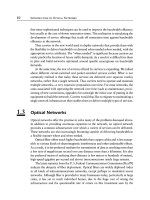
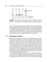
Figure 1.3 Bandwidth growth over time in different types of networks.
service providers. Before providing some more data, we introduce some terminology

first. Each
route
in a network comprises many fiber
cables.
Each cable contains many
fibers.
For example, a 10-mile-long route using 3 fiber cables is said to have 10 route
miles and 30
sheath
(cable) miles. If each cable has 20 fibers, the same route is said to
have 600 fiber miles. As of the end of 1998, the local-exchange carriers in the United
States had deployed more than 355,000 sheath miles of fiber, containing more than
16 million fiber miles. More than 160,000 route miles of fiber had been deployed
by the interexchange carriers in the United States, containing more than 3.6 million
miles of optical fiber [Kra99].
Fiber transmission technology has evolved over the past few decades to offer
higher and higher bit rates on a fiber over longer and longer distances. Figure 1.3
plots the growth in bandwidth over time of different types of networks, updated
from a chart originally presented in [Fra93]. This tremendous growth in bandwidth
is primarily due to the deployment of optical fiber communication systems.
Note from Figure 1.3 that the bandwidths into our homes are still limited by the
bandwidth available on our phone line, which is made of twisted-pair copper cable.
These lines are capable of carrying data at a few megabits per second using digital
subscriber loop (DSL) technology, but voice-grade lines are limited at the central
office to 4 kHz of bandwidth. (Note that in some cases we measure bandwidth in
hertz and sometimes loosely use bit rates when talking about bandwidth. We will
12 INTRODUCTION TO OPTICAL NETWORKS
1.3.1
quantify the relationship between bit rate and bandwidth in Section 1.7.) The other
alternative is the cable network, which again is capable of providing a few megabits

per second to each subscriber on a shared basis using cable modem technology.
When we talk about optical networks, we are really talking about two gener-
ations of optical networks. In the first generation, optics was essentially used for
transmission and simply to provide capacity. Optical fiber provided lower bit error
rates and higher capacities than copper cables. All the switching and other intelligent
network functions were handled by electronics. Examples of first-generation optical
networks are SONET (synchronous optical network) and the essentially similar SDH
(synchronous digital hierarchy) networks, which form the core of the telecommuni-
cations infrastructure in North America and in Europe and Asia, respectively, as well
as a variety of enterprise networks such as ESCON (enterprise serial connection).
We will study these first-generation networks in Chapter 6.
Today we are seeing the deployment of second-generation optical networks,
where some of the routing, switching, and intelligence is moving into the
optical
layer.
Before we discuss this new generation of networks, we will first look at the
multiplexing techniques that provide the capacity needed to realize these networks.
Multiplexing Techniques
The need for multiplexing is driven by the fact that it is much more economical
to transmit data at higher rates over a single fiber than it is to transmit at lower
rates over multiple fibers, in most applications. There are fundamentally two ways
of increasing the transmission capacity on a fiber, as shown in Figure 1.4. The first
is to increase the bit rate. This requires higher-speed electronics. Many lower-speed
data streams are multiplexed into a higher-speed stream at the transmission bit rate
by means of electronic
time division multiplexing
(TDM). The multiplexer typically
interleaves the lower-speed streams to obtain the higher-speed stream. For example,
it could pick 1 byte of data from the first stream, the next byte from the second
stream, and so on. As an example, 64 155 Mb/s streams may be multiplexed into a

single 10 Gb/s stream. Today, the highest transmission rate in commercially available
systems is around 10 Gb/s; 40 Gb/s TDM technology will be available soon. To
push TDM technology beyond these rates, researchers are working on methods to
perform the multiplexing and demultiplexing functions
optically.
This approach is
called
optical time division multiplexing
(OTDM). Laboratory experiments have
demonstrated the multiplexing/demultiplexing of several 10 Gb/s streams into/from
a 250 Gb/s stream, although commercial implementation of OTDM is still several
years away. We will study OTDM systems in Chapter 12. However, multiplexing
and demultiplexing high-speed streams by itself is not sufficient to realize practical
networks. We need to contend with the various impairments that arise as these very
1.3 Optical Networks
13
Figure
1.4 Different multiplexing techniques for increasing the transmission capacity
on an optical fiber. (a) Electronic or optical time division multiplexing and (b) wavelength
division multiplexing. Both multiplexing techniques take in N data streams, each of B b/s,
and multiplex them into a single fiber with a total aggregate rate of
NB
b/s.
high-speed streams are transmitted over a fiber. As we will see in Chapters 5 and 13,
the higher the bit rate, the more difficult it is to engineer around these impairments.
However, similar bottlenecks have been encountered in the past, and people have
always found ways to overcome them; so we can expect the transmission bit rates
to continue to increase, although perhaps not at the breakneck pace of the past two
decades.
Another way to increase the capacity is by a technique called

wavelength division
multiplexing
(WDM). WDM is essentially the same as frequency division multiplex-
ing (FDM), which has been used in radio systems for more than a century. For some
reason, the term FDM is used widely in radio communication, but WDM is used in
14 INTRODUCTION TO OPTICAL NETWORKS
1.3.2
the context of optical communication, perhaps because FDM was studied first by
communications engineers and WDM by physicists. The idea is to transmit data si-
multaneously at multiple carrier wavelengths (or, equivalently, frequencies or colors)
over a fiber. To first order, these wavelengths do not interfere with each other pro-
vided they are kept sufficiently far apart. (There are some undesirable second-order
effects where wavelengths do interfere with each other, and we will study these in
Chapters 2 and 5.) Thus WDM provides
virtual fibers,
in that it makes a single
fiber look like multiple "virtual" fibers, with each virtual fiber carrying a single
data stream. WDM systems are widely deployed today in long-haul and undersea
networks and are being deployed in metro networks as well.
WDM and TDM both provide ways to increase the transmission capacity and
are complementary to each other. Therefore networks today use a combination
of TDM and WDM. The question of what combination of TDM and WDM to
use in systems is an important one facing carriers today. For example, suppose a
carrier wants to install an 80 Gb/s link. Should we deploy 32 WDM channels at
2.5 Gb/s each or should we deploy 10 WDM channels at 8 Gb/s each? The answer
depends on a number of factors, including the type and parameters of the fiber
used in the link and the services that the carrier wishes to provide using that link.
We will discuss this issue in Chapter 13. Using a combination of WDM and TDM,
systems with transmission capacities of around I Tb/s over a single fiber are becoming
commercially available, and no doubt we will see systems with higher capacities

operating over longer distances emerge in the future.
Second-Generation Optical Networks
Optics is clearly the preferred means of transmission, and WDM transmission is now
widely used in the network. In recent years, people have realized that optical networks
are capable of providing more functions than just point-to-point transmission. Major
advantages are to be gained by incorporating some of the switching and routing
functions that were performed by electronics into the optical part of the network. For
example, as data rates get higher and higher, it becomes more difficult for electronics
to process data. Suppose the electronics must process data in blocks of 53 bytes
each (this happens to be the block size in asynchronous transfer mode networks). In
a 100 Mb/s data stream, we have 4.24 lZS to process a block, whereas at 10 Gb/s,
the same block must be processed within 42.4 ns. In first-generation networks, the
electronics at a node must handle not only all the data intended for that node but
also all the data that is being passed through that node on to other nodes in the
network. If the latter data could be routed through in the optical domain, the burden
on the underlying electronics at the node would be significantly reduced. This is one
of the key drivers for second-generation optical networks.
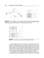
1.3 Optical Networks 15
Optical networks based on this paradigm are now being deployed. The ar-
chitecture of such a network is shown in Figure 1.5. We call this network a
wavelength-routing
network. The network provides
lightpaths
to its users, such
as SONET terminals or IP routers. Lightpaths are optical connections carried end to
end from a source node to a destination node over a wavelength on each intermediate
link. At intermediate nodes in the network, the lightpaths are routed and switched
from one link to another link. In some cases, lightpaths may be converted from one
wavelength to another wavelength as well along their route. Different lightpaths in
a wavelength routing network can use the same wavelength as long as they do not

share any common links. This allows the same wavelength to be reused spatially in
different parts of the network. For example, Figure 1.5 shows six lightpaths. The
lightpath between B and C, the lightpath between D and E, and one of the lightpaths
between E and F do not share any links in the network and can therefore be set
up using the same wavelength )~1. At the same time, the lightpath between A and F
shares a link with the lightpath between B and C and must therefore use a different
wavelength. Likewise, the two lightpaths between E and F must be assigned different
wavelengths. Note that these lightpaths all use the same wavelength on every link in
their path. This is a constraint that we must deal with if we do not have
wavelength
conversion
capabilities within the network. Suppose we had only two wavelengths
available in the network and wanted to set up a new lightpath between nodes E and
E Without wavelength conversion, we would not be able to set up this lightpath. On
the other hand, if the intermediate node X can perform wavelength conversion, then
we can set up this lightpath using wavelength )~2 on link EX and wavelength ~1 on
link XE
The key network elements that enable optical networking are
optical line ter-
minals
(OLTs),
optical add~drop multiplexers
(OADMs), and
optical crossconnects
(OXCs), as shown in Figure 1.5. An OLT multiplexes multiple wavelengths into a
single fiber and demultiplexes a set of wavelengths on a single fiber into separate
fibers. OLTs are used at the ends of a point-to-point WDM link. An OADM takes
in signals at multiple wavelengths and selectively drops some of these wavelengths
locally while letting others pass through. It also selectively adds wavelengths to the
composite outbound signal. An OADM has two

line
ports where the composite
WDM signals are present, and a number of
local
ports where individual wavelengths
are dropped and added. An OXC essentially performs a similar function but at
much larger sizes. OXCs have a large number of ports (ranging from a few tens
to thousands) and are able to switch wavelengths from one input port to another.
Both OADMs and OXCs may incorporate wavelength conversion capabilities. The
detailed architecture of these networks will be discussed in Chapter 7.
Optical networks based on the architecture described above are already being
deployed. OLTs have been widely deployed for point-to-point applications. OADMs
16 INTRODUCTION TO OPTICAL NETWORKS
Figure 1.5 A
WDM wavelength-routing network, showing optical line terminals
(OLTs), optical add/drop multiplexers (OADMs), and optical crossconnects (OXCs).
The network provides lightpaths to its users, which are typically IP routers or SONET
terminals.
are now used in long-haul and metro networks. OXCs are beginning to be deployed
first in long-haul networks because of the higher capacities in those networks.
1.4
The Optical Layer
Before delving into the details of the optical layer, we first introduce the notion of
a layered network architecture. Networks are complicated entities with a variety of
different functions being performed by different components of the network, with
equipment from different vendors all interworking together. In order to simplify our
view of the network, it is desirable to break up the functions of the network into
different layers, as shown in Figure 1.6. This type of layered model was proposed
by the International Standards Organization (ISO) in the early 1980s. Imagine the
layers as being vertically stacked up. Each layer performs a certain set of functions

1.4 The Optical Layer 17
Figure 1.6
(NE).
Layered hierarchy of a network showing the layers at each network element
and provides a certain set of services to the next higher layer. In turn, each layer
expects the layer below it to deliver a certain set of services to it. The service interface
between two adjacent layers is called a
service access point
(SAP), and there can be
multiple SAPs between layers corresponding to different types of services offered.
In most cases, the network provides
connections
to the user. A connection is
established between a source and a destination node. Setting up, taking down, and
managing the state of a connection is the job of a separate network control and
management entity (not shown in Figure 1.6), which may control each individual
layer in the network. There are also examples where the network provides
con-
nectionless
services to the user. These services are suitable for transmitting short
messages across a network, without having to pay the overhead of setting up and
taking down a connection for this purpose. We will confine the following discussion
to the connection-oriented model.
Within a network element, data belonging to a connection flows between the
layers. Each layer multiplexes a number of higher-layer connections and may add
some additional overhead to data coming from the higher layer. Each intermediate
network element along the path of a connection embodies a set of layers starting
from the lowest layer up to a certain layer in the hierarchy.
18 INTRODUCTION TO OPTICAL NETWORKS
Figure

1.7 The classical layered hierarchy.
It is imi0ortant to define the functions of each layer and the interfaces between
layers. This is essential because it allows vendors to manufacture a variety of hard-
ware and software products performing the functions of some, but not all, of the
layers, and provide the appropriate interfaces to communicate with other products
performing the functions of other layers.
There are many possible implementations and standards for each layer. A given
layer may work together with a variety of lower or higher layers. Each of the different
types of optical networks that we will study constitutes a layer. Each layer itself can
in turn be broken up into several sublayers. As we study these networks, we will
explore this layered hierarchy further.
Figure 1.7 shows a classical breakdown of the different layers in a network that
was proposed by the International Standards Organization. The lowest layer in the
hierarchy is the
physical layer,
which provides a "pipe" with a certain amount of
bandwidth to the layer above it. The physical layer may be optical, wireless, or coaxial
or twisted-pair cable. The next layer above is the
data link layer,
which is responsible
for framing, multiplexing, and demultiplexing data sent over the physical layer. The
framing protocol defines how data is transported over a physical link. Typically
data is broken up into frames before being transmitted ove~ a physical link. This is
necessary to ensure reliable delivery of data across the link. The framing protocol
provides clear delineation between frames, provides sufficient transitions in the signal
so that it can be recovered at the other end, and usually includes additional overhead
that enables link errors to be detected. Examples of data link protocols suitable for
operation over point-to-point links include the
point-to-point protocol
(PPP) and the

high-level data link control
(HDLC) protocol. Included in the data link layer is the
1.4 The Optical Layer 19
media access control layer
(MAC), which coordinates the transmissions of different
nodes when they all share common bandwidth, as is the case in many local-area
networks, such as Ethernets and token rings.
Above the data link layer resides the
network layer.
The network layer usually
provides
virtual circuits
or
datagram
services to the higher layer. A virtual circuit
(VC) represents an end-to-end connection with a certain set of quality-of-service
parameters associated with it, such as bandwidth and error rate. Data transmitted
by the source over a VC is delivered in sequence at its destination. Datagrams, on
the other hand, are short messages transmitted end to end, with no notion of a
connection. The network layer performs the end-to-end routing function of taking a
message at its source and delivering it to its destination. The predominant network
layer today is IP, and the main network element in an IP network is an IP router.
IP provides a way to route packets (or datagrams) end to end in a packet-switched
network. IP includes statistical multiplexing of multiple packet streams and today
also provides some simple and relatively slow and inefficient service restoration
mechanisms. The Internet Protocol has been adapted to operate over a variety of
data link and physical media, such as Ethernet, serial telephone lines, coaxial cable
lines, and optical fiber lines.
The
transport layer

resides on top of the network layer and is responsible for
ensuring the end-to-end, in-sequence, and error-free delivery of the transmitted mes-
sages. For example, the
transmission control protocol
(TCP) used in the Internet
belongs to this layer. Above the transport layer reside other layers such as the
ses-
sion, presentation,
and
application
layers, but we will not be concerned with these
layers in this book.
Another important packet-switched layer is ATM. ATM provides a connection-
oriented service (virtual circuits) and is capable of providing a variety of
quality-of-service guarantees. Packets in ATM are called
cells
and are of fixed
length (53 bytes). ATM is being used by many carriers as a vehicle to deliver re-
liable packet-switched services. More on this subject in Chapters 6 and 13.
This classical layered view of networks needs some embellishment to handle the
variety of networks and protocols that are proliferating today. A more realistic lay-
ered model for today's networks would employ multiple protocol stacks residing
one on top of the other. Each stack incorporates several sublayers, which may pro-
vide functions resembling traditional physical, link, and network layers. To provide
a concrete example of this, consider an IP over SONET network shown in Fig-
ure 1.8. In this case, the IP network treats the SONET network as providing it with
point-to-point links between IP routers. The SONET layer itself, however, internally
routes and switches connections, and in a sense, incorporates its own link, physical,
and network layers.