Optical Networks: A Practical Perspective - Part 6 pdf

20 INTRODUCTION TO OPTICAL NETWORKS
Figure 1.8 An IP over SONET network. (a) The network has IP switches with SONET adaptors
that are connected to a SONET network. (b) The layered view of this network.
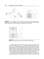
Figure 1.9 The layered view of an IP over ATM over SONET network.
Another example of this sort of layering arises in the context of an IP over
ATM over SONET network. Some service providers are deploying an ATM network
operating over a SONET infrastructure to provide services for IP users. In such a
network, IP packets are converted to ATM cells at the periphery of the network. The
ATM switches are connected through a SONET infrastructure. The layered view
of such a network is shown in Figure 1.9. Again, the IP network treats the ATM
network as its link layer, and the ATM network uses SONET as its link layer.
The introduction of second-generation optical networks adds yet another layer to
the protocol hierarchy the so-called optical layer. The optical layer is a
server
layer
1.4 The Optical Layer
21
Figure
1.10 A layered view of a network consisting of a second-generation optical
network layer that supports a variety of client layers above it.
that provides services to other
client
layers. This optical layer provides lightpaths
to a variety of client layers, as shown in Figure 1.10. Examples of client layers
residing above a second-generation optical network layer include IP, ATM, and
SONET/SDH, as well as other possible protocols such as Gigabit Ethernet, ESCON
(enterprise serial connection~a protocol used to interconnect computers to storage
devices and other computers), or Fibre Channel (which performs the same function
as ESCON, at higher speeds). As second-generation optical networks evolve, they
may provide other services besides lightpaths, such as packet-switched virtual circuit
or datagram services. These services may directly interface with user applications, as

shown in Figure 1.10. Several other layer combinations are possible and not shown
in the figure, such as IP over SONET over optical, and ATM over optical.
The client layers make use of the lightpaths provided by the optical layer. To a
SONET network operating over the optical layer, the lightpaths are simply replace-
ments for hardwired fiber connections between SONET terminals. As described
earlier, a lightpath is a connection between two nodes in the network, and it is set
up by assigning a dedicated wavelength to it on each link in its path. Note that
individual wavelengths are likely to carry data at fairly high bit rates (a few gigabits
per second), and this entire bandwidth is provided to the higher layer by a lightpath.
Depending on the capabilities of the network, this lightpath could be set up or taken
down in response to a request from the higher layer. This can be thought of as a
circuit-switched
service, akin to the service provided by today's telephone network:
the network sets up or takes down calls in response to a request from the user. Al-
ternatively, the network may provide only
permanent
lightpaths, which are set up
22 INTRODUCTION TO OPTICAL NETWORKS
at the time the network is deployed. This lightpath service can be used to support
high-speed connections for a variety of overlying networks.
Optical networks today provide functions that might be thought of as falling
primarily within the physical layer from the perspective of its users. However, the
optical network itself incorporates several sublayers, which in turn correspond to
the link and network layer functions in the classical layered view.
Before the emergence of the optical layer, SONET/SDH was the predominant
transmission layer in the telecommunications network, and it is still the dominant
layer in many parts of the network. We will study SONET/SDH in detail in Chap-
ter 6. For convenience, we will use SONET terminology in the rest of this section.
The SONET layer provides several key functions. It provides end-to-end, managed,
circuit-switched connections. It provides an efficient mechanism for multiplexing

lower-speed connections into higher-speed connections. For example, low-speed
voice connections at 64 kb/s or private line 1.5 Mb/s connections can be multiplexed
all the way up into 2.5 Gb/s or 10 Gb/s line rates for transport over the network.
Moreover, at intermediate nodes, SONET provides an efficient way to extract indi-
vidual low-speed streams from a high-speed stream, using an elegant multiplexing
mechanism based on the use of pointers.
SONET also provides a high degree of network reliability and availability. Car-
riers expect their networks to provide 99.99% to 99.999% of availability. These
numbers translate into an allowable network downtime of less than one hour per
year and five minutes per year, respectively. SONET achieves this by incorporating
sophisticated mechanisms for rapid service restoration in the event of failures in the
network. This is a subject we will look at in Chapter 10.
Finally, SONET includes extensive overheads that allow operators to monitor
and manage the network. Examples of these overheads include parity check bytes
to determine whether frames are received in error or not, and connection identifiers
that allow connections to be traced and verified across a complex network.
SONET network elements include line terminals, add/drop multiplexers (ADMs),
regenerators, and digital crossconnects (DCSs). Line terminals multiplex and demul-
tiplex traffic streams. ADMs are deployed in linear and ring network configurations.
They provide an efficient way to drop part of the traffic at a node while allowing
the remaining traffic to pass through. The ring topology allows traffic to be rerouted
around failures in the network. Regenerators regenerate the SONET signal wherever
needed. DCSs are deployed in larger nodes to switch a large number of traffic streams.
Today's DCSs are capable of switching thousands of 45 Mb/s traffic streams.
The functions performed by the optical layer are in many ways analogous to those
performed by the SONET layer. The optical layer multiplexes multiple lightpaths into
a single fiber and allows individual lightpaths to be extracted efficiently from the
composite multiplex signal at network nodes. It incorporates sophisticated service
1.4 The Optical Layer 23
Figure

1.11 Example of a typical multiplexing layered hierarchy.
restoration techniques and management techniques as well. We will look at these
techniques in Chapters 9 and 10.
Figure 1.11 shows a typical layered network hierarchy, highlighting the optical
layer. The optical layer provides lightpaths that are used by SONET and IP network
elements. The SONET layer multiplexes low-speed circuit-switched streams into
higher-speed streams, which are then carried over lightpaths. The IP layer performs
statistical multiplexing of packet-switched streams into higher-speed streams, which
are also carried over lightpaths. Inside the optical layer itself is a multiplexing hi-
erarchy. Multiple wavelengths or lightpaths are combined together into wavelength
bands. Bands are combined together to produce a composite WDM signal on a fiber.
The network itself may include multiple fibers and multiple fiber bundles, each of
which carries a number of fibers.
So why have multiple layers in the network that perform similar functions? The
answer is that this form of layering significantly reduces network equipment costs.
Different layers are more efficient at performing functions at different bit rates.
For example, the SONET layer can efficiently (that is, cost-effectively) switch and
process traffic streams up to, say, 2.5 Gb/s today. However, it is very expensive
to have this layer process 100 10 Gb/s streams coming in on a WDM link. The
optical layer, on the other hand, is particularly efficient at processing traffic on
a wavelength-by-wavelength basis, but not particularly good at processing traffic
streams at lower granularities, for example, 155 Mb/s. Therefore, it makes sense to
use the optical layer to process large amounts of bandwidth at a relatively coarse level
and the SONET layer to process smaller amounts of bandwidth at a relatively finer
24 INTRODUCTION TO OPTICAL NETWORKS
level. This fundamental observation is the key driver to providing such functions in
multiple layers, and we will study this in detail in Chapter 7.
A similar observation also holds for the service restoration function of these
networks. Certain failures are better handled by the optical layer and certain others
by the SONET layer or the IP layer. We will study this aspect in Chapter 10.

1.5
Transparency and All-Optical Networks
A major feature of the lightpath service provided by second-generation networks is
that this type of service can be
transparent
to the actual data being sent over the
lightpath once it is set up. For instance, a certain maximum and minimum bit rate
might be specified, and the service may accept data at any bit rate and any protocol
format within these limits. It may also be able to carry analog data.
Transparency in the network provides several advantages. An operator can pro-
vide a variety of different services using a single infrastructure. We can think of this
as
service transparency.
Second, the infrastructure is future-proof in that if protocols
or bit rates change, the equipment deployed in the network is still likely to be able to
support the new protocols and/or bit rates without requiring a complete overhaul of
the entire network. This allows new services to be deployed efficiently and rapidly,
while allowing legacy services to be carried as well.
An example of a transparent network of this sort is the telephone network. Once
a call is established in the telephone network, it provides 4 kHz of bandwidth over
which a user can send a variety of different types of traffic such as voice, data, or
fax. There is no question that transparency in the telephone network today has had
a far-reaching impact on our lifestyles. Transparency has become a useful feature of
second-generation optical networks as well.
Another term associated with transparent networks is the notion of an
all-optical
network.
In an all-optical network, data is carried from its source to its destination in
optical form, without undergoing any optical-to-electrical conversions along the way.
In an ideal world, such a network would be

fully transparent.
However, all-optical
networks are limited in their scope by several parameters of the physical layer, such
as bandwidth and signal-to-noise ratios. For example, analog signals require much
higher signal-to-noise ratios than digital signals. The actual requirements depend on
the modulation format used as well as the bit rate. We will study these aspects in
Chapter 5, where we will see that engineering the physical layer is a complex task
with a variety of parameters to be taken into consideration. For this reason, it is very
difficult to build and operate a network that can support analog as well as digital
signals at arbitrary bit rates.
1.5 Transparency and All-Optical Networks
25
The other extreme is to build a network that handles essentially a single bit rate
and protocol (say, 2.5 Gb/s SONET only). This would be a
nontransparent
network.
In between is a
practical
network that handles digital signals at a range of bit rates
up to a specified maximum. Most optical networks being deployed today fall into
this category.
Although we talk about optical networks, they almost always include a fair
amount of electronics. First, electronics plays a crucial role in performing the intelli-
gent control and management functions within a network. However, even in the data
path, in most cases, electronics is needed at the periphery of the network to adapt
the signals entering the optical network. In many cases, the signal may not be able
to remain in optical form all the Way to its destination due to limitations imposed by
the physical layer design and may have to be regenerated in between. In other cases,
the signal may have to be converted from one wavelength to another wavelength.
In all these situations, the signal is usually converted from optical form to electronic

form and back again to optical form'
Having these electronic regenerators in the path of the signal reduces the trans-
parency of that path. There are three types of electronic regeneration techniques for
digital data. The standard one is called regeneration
with
retiming and reshaping,
also known as 3R. Here the bit clock is extracted from the signal, and the signal is
reclocked. This technique essentially produces a "fresh" copy of the signal at each
regeneration step, allowing the signal to go through a very large number of regen-
erators. However, it eliminates transparency to bit rates and the framing protocols,
since acquiring theclock usually requires knowledge of both of these. Some limited
form of bit rate transparency is possible by making use of programmable clock re-
covery chips that can work at a set of bit rates that are multiples of one another. For
example, chipsets that perform clock recovery at either 2.5 Gb/s or 622 Mb/s are
commercially available today.
An implementation using regeneration of the optical signal
without
retiming,
also called 2R, offers transparency to bit rates, without supporting analog data or
different modulation formats [GJR96]. However, this approach limits the number
of regeneration steps allowed, particularly at higher bit rates, over a few hundred
megabits per second. The limitation is due to the jitter, which accumulates at each
regeneration step.
The final form of electronic regeneration is 1R, where the signal is simply received
and retransmitted without retiming or reshaping. This form of regeneration can
handle analog data as well, but its performance is significantly poorer than the other
two forms of regeneration. For this reason, the networks being deployed today use
2R or 3R electronic regeneration. Note, however, that optical amplifiers are widely
used to amplify the signal in the optical domain, without converting the signal to the
electrical domain. These can be thought of as 1R optical regenerators.

26
INTRODUCTION TO OPTICAL NETWORKS
Table
1.1 Different types of transparency in an optical network.
Transparency type
Parameter Fully transparent Practical Nontransparent
Analog/digital Both Digital Digital
Bit rate Arbitrary Predetermined maximum Fixed
Framing protocol Arbitrary Selected few Single
Table 1.1 provides an overview of the different dimensions of transparency. At
one end of the spectrum is a network that operates at a fixed bit rate and framing
protocol, for example, SONET at 2.5 Gb/s. This would be truly an
opaque network.
In contrast, a fully transparent network would support analog and digital signals
with arbitrary bit rates and framing protocols. As we argued earlier, however, such
a network is not practical to engineer and build. Today, a practical alternative is
to engineer the network to support a variety of digital signals up to a predeter-
mined maximum bit rate and a specific set of framing protocols, such as SONET
and Gigabit Ethernet. The network supports a variety of framing protocols either
by making use of 2R regeneration inside the network or by providing specific 3R
adaptation devices for each of the framing protocols. Such a network is shown in
Figure 1.12. It can be viewed as consisting of islands of all-optical subnetworks
with optical-to-electrical-to-optical conversion at their boundaries for the purposes
of adaptation, regeneration, or wavelength conversion.
1.6
Optical Packet Switching
So far we have talked about optical networks that provide lightpaths. These networks
are essentially circuit-switched. Researchers are also working on optical networks
that can perform packet switching in the optical domain. Such a network would be
able to offer

virtual circuit services or datagram services, much like what is provided
by ATM and IP networks. With a virtual circuit connection, the network offers what
looks like a circuit-switched connection between two nodes. However, the band-
width offered on the connection can be smaller than the full bandwidth available
on a link or wavelength. For instance, individual connections in a future high-speed
network may operate at 10 Gb/s, while transmission bit rates on a wavelength could
be 100 Gb/s. Thus the network must incorporate some form of time division mul-
tiplexing to combine multiple connections onto the transmission bit rate. At these
rates, it may be easier to do the multiplexing in the optical domain rather than in
the electronic domain. This form of optical time domain multiplexing (OTDM) may
1.6 Optical Packet Switching
27
Figure
1.12 An optical network consisting of all-optical subnetworks interconnected
by optical-to-electrical-to-optical (OEO) converters. OEO converters are used in the
network for adapting external signals to the optical network, for regeneration, and for
wavelength conversion.
be
fixed
or
statistical.
Those that perform statistical multiplexing are called optical
packet-switched networks. For simplicity we will talk mostly about optical packet
switching. Fixed OTDM can be thought of as a subset of optical packet switching
where the multiplexing is fixed instead of statistical.
An optical packet-switching node is shown in Figure 1.13. The idea is to create
packet-switching nodes with much higher capacities than can be envisioned with
electronic packet switching. Such a node takes a packet coming in, reads its header,
and switches it to the appropriate output port. The node may also impose a new
header on the packet. It must also handle

contention
for output ports. If two packets
coming in on different ports need to go out on the same output port, one of the
packets must be buffered, or sent out on another port.
Ideally, all the functions inside the node would be performed in the optical do-
main, but in practice, certain functions, such as processing the header and controlling
the switch, get relegated to the electronic domain. This is because of the very limited
processing capabilities in the optical domain. The header itself could be sent at a
lower bit rate than the data so that it can be processed electronically.
The mission of optical packet switching is to enable packet-switching capabilities
at rates that cannot be contemplated using electronic packet switching. However,
designers are handicapped by several limitations with respect to processing signals
in the optical domain. One important factor is the lack of optical random access
28
INTRODUCTION TO OPTICAL NETWORKS
Figure 1.13 An optical packet-switching node. The node buffers the incoming packets,
looks at the packet header, and routes the packets to an appropriate output port based
on the information contained in the header.
memory for buffering. Optical buffers are realized by using a length of fiber
and
are just simple delay lines, not fully functional memories. Packet switches include a
high amount of intelligent real-time software and dedicated hardware to control the
network and provide quality-of-service guarantees, and these functions are ,difficult
to perform in the optical domain. Another factor is the relatively primitive state of
fast optical-switching technology, compared to electronics. For these reasons, optical
packet switching is still in its infancy today in research laboratories. Chapter 12
covers all these aspects in detail.
1.7
Transmission Basics
In this section, we introduce and define the units for common parameters associated

with optical communication systems.
1.7.1
Wavelengths, Frequencies, and Channel Spacing
When we talk about WDM signals, we will be talking about the wavelength, or
frequency, of these signals. The wavelength )~ and frequency f are related by the
equation
c=f~.,
where c denotes the speed of light in free space, which is 3 x 108 m/s. We will reference
all parameters to free space. The speed of light in fiber is actually somewhat lower
(closer to 2 x 108 m/s), and the wavelengths are also correspondingly different.
1.7 Transmission Basics
29
To characterize a WDM signal, we can use either its frequency or wavelength in-
terchangeably. Wavelength is measured in units of nanometers (nm) or micrometers
(#m or microns). (1 nm = 10 -9 m, 1 #m = 10 -6 m.) The wavelengths of interest
to optical fiber communication are centered around 0.8, 1.3, and 1.55 ~m. These
wavelengths lie in the infrared band, which is not visible to the human eye. Frequen-
cies are measured in units of hertz (or cycles per second), more typically in megahertz
(1 MHz = 106 Hz), gigahertz (1 GHz = 109 Hz), or terahertz (1 THz = 1012 Hz).
Using c - 3 • 108 m/s, a wavelength of 1.55 #m would correspond to a frequency
of approximately 193 THz, which is 193 • 1012 Hz.
Another parameter of interest is the channel spacing, which is the spacing between
two wavelengths or frequencies in a WDM system. Again the channel spacing can be
measured in units of wavelengths or frequencies. The relationship between the two
can be obtained starting from the equation
C
f ~ o
Differentiating this equation around a center wavelength )~0, we obtain the relation-
ship between the frequency spacing Af and the wavelength spacing A)~ as
r

Af ) ~ A)~.
This relationship is accurate as long as the wavelength (or frequency) spacing is small
compared to the actual channel wavelength (or frequency), which is usually the case
in optical communication systems. At a wavelength )~0 = 1550 nm, a wavelength
spacing of 0.8 nm corresponds to a frequency spacing of 100 GHz, a typical spacing
in WDM systems.
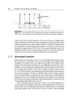
Digital information signals in the time domain can be viewed as a periodic se-
quence of pulses, which are on or off, depending on whether the data is a 1 or a
0. The bit rate is simply the inverse of this period. These signals have an equivalent
representation in the frequency domain, where the energy of the signal is spread
across a set of frequencies. This representation is called the
power spectrum, or sim-
ply
spectrum. The signal bandwidth is a measure of the width of the spectrum of the
signal. The bandwidth can also be measured either in the frequency domain or in
the wavelength domain, but is mostly measured in units of frequency. Note that we
have been using the term
bandwidth rather loosely. The bandwidth and bit rate of a
digital signal are related but not exactly the same. Bandwidth is usually specified in
kilohertz or megahertz or gigahertz, whereas bit rate is specified in kilobits/second
(kb/s), megabits/second (Mb/s), or gigabits/second (Gb/s). The relationship between
the two depends on the type of modulation used. For instance, a phone line offers
4 kHz of bandwidth, but sophisticated modulation technology allows us to realize