Optical Networks: A Practical Perspective - Part 7 pdf

30
INTRODUCTION TO OPTICAL NETWORKS
00 GH 00 GH
I
TM
Vl-~ r
k
" 1 bandwidth
193.3 193.2 193.1 193.0 192.9 Frequency (THz)
1550.918 1551.721 1552.524 1553.329 1554.134 Wavelength(nm)
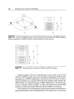
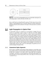
Figure 1.14 The 100 GHz ITU frequency grid based on a reference frequency of
193.1 THz. A 50 GHz grid has also been defined around the same reference frequency.
a bit rate of 56 kb/s over this phone line. This ratio of bit rate to available band-
width is called
spectral efficiency.
Optical communication systems use rather simple
modulation techniques that achieve a spectral efficiency of about 0.4 bits/s/Hz, and
it is reasonable to assume therefore that a signal at a bit rate of 10 Gb/s uses up
bandwidth of approximately 25 GHz. Note that the signal bandwidth needs to be
sufficiently smaller than the channel spacing; otherwise we would have undesirable
interference between adjacent channels and distortion of the signal itself.
1.7.2
Wavelength Standards
WDM systems today primarily use the 1.55 >m wavelength region for two reasons:
the inherent loss in optical fiber is the lowest in that region, and excellent optical
amplifiers are available in that region. We will discuss this in more detail in later
chapters. The wavelengths and frequencies used in WDM systems have been stan-
dardized on a frequency grid by the International Telecommunications Union (ITU).
It is an infinite grid centered at 193.1 THz, a segment of which is shown in Fig-
ure 1.14. The ITU decided to standardize the grid in the frequency domain based on
equal channel spacings of 50 GHz or 100 GHz. Observe that if multiple channels

are spaced apart equally in wavelength, they are not spaced apart exactly equally in
frequency, and vice versa. The figure also shows the power spectrum of two channels
400 GHz apart in the grid populated by traffic-bearing signals, as indicated by the
increased signal bandwidth on those channels.
The ITU grid only tells part of the story. Today, we are already starting to see
systems using 25 GHz channel spacings. We are also seeing the use of several trans-
mission bands. The early WDM systems used the so-called C-band, or conventional
band (approximately 1530-1565 nm). The use of the L-band, or long wavelength
1.7 Transmission Basics 31
band (approximately 1565-1625 nm), has become feasible recently with the devel-
opment of optical amplifiers in this band. We will look at this and other bands in
Section 1.8.
It has proven difficult to obtain agreement from the different WDM vendors and
service providers on more concrete wavelength standards. As we will see in Chap-
ters 2 and 5, designing WDM transmission systems is a complex endeavor, requiring
trade-offs among many different parameters, including the specific wavelengths used
in the system. Different WDM vendors use different methods for optimizing their
system designs, and converging on a wavelength plan becomes difficult as a result.
However, the ITU grid standard has helped accelerate the deployment of WDM sys-
tems because component vendors can build wavelength-selective parts to a specific
grid, which helps significantly in inventory management and manufacturing.
1.7.3
Optical Power and Loss
In optical communication, it is quite common to use decibel units (dB) to measure
power and signal levels, as opposed to conventional units. The reason for doing this
is that powers vary over several orders of magnitude in a system, and this makes it
easier to deal with a logarithmic rather than a linear scale. Moreover, by using such
a scale, calculations that involve multiplication in the conventional domain become
additive operations in the decibel domain. Decibel units are used to represent relative
as well as absolute values.

To understand this system, let us consider an optical fiber link. Suppose we
transmit a light signal with power
Pt
watts (W). In terms of dB units, we have
( Pt
)dBW =
10 log(Pt)w.
In many cases, it is more convenient to measure powers in milliwatts (mW), and we
have an equivalent dBm value given as
( Pt
)dBm 10 log(Pt )mW.
For example, a power of 1 mW corresponds to 0 dBm or -30 dBW. A power of
10 mW corresponds to 10 dBm or -20 dBW.
As the light signal propagates through the fiber, it is attenuated; that is, its power
is decreased. At the end of the link, suppose the received power is P~. The link loss
y is then defined as
P~
y no
Pt
32
INTRODUCTION TO OPTICAL NETWORKS
In dB units, we would have
(Y)dB =
10 log g = (Pr)dBm
(Pt)dBm-
Note that dB is used to indicate relative values, whereas dBm and dBW are used to
indicate the absolute power value. As an example, if Pt = 1 mW and Pr = 1 /~W,
implying that y = 0.001, we would have, equivalently,
(et)dBm = 0
dBm or - 30 dBW,

(er)dBm =
-30 dBm or - 60 dBW,
and
(Y)dB = 30 dB.
In this context, a signal being attenuated by a factor of 1000 would equivalently
undergo a 30 dB loss. A signal being amplified by a factor of 1000 would equivalently
have a 30 dB gain.
We measure loss in optical fiber usually in units of dB/km. So, for example, a
light signal traveling through 120 km of fiber with a loss of 0.25 dB/km would be
attenuated by 30 dB.
1.8
Network Evolution
We conclude this chapter by outlining the trends and factors that have shaped the
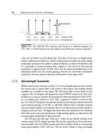
evolution of optical fiber transmission systems and networks. Figure 1.15 gives an
overview. The history of optical fiber transmission has been all about how to transmit
data at the highest capacity over the longest possible distance and is remarkable for
its rapid progress. What is equally remarkable is the fact that researchers have
successfully overcome numerous obstacles along this path, many of which when first
discovered looked as though they would impede further increases in capacity and
transmission distance. The net result of this is that capacity continues to grow in
the network, while the cost per bit transmitted per kilometer continues to get lower
and lower, to a point where it has become practical for carriers to price circuits
independently of the distance.
We will introduce various types of fiber propagation impairments as well as
optical components in this section. These will be covered in depth in Chapters 2, 3,
and 5.
1.8 Network Evolution 33
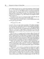
Figure 1.15 Evolution of optical fiber transmission systems. (a) An early system using LEDs over
multimode fiber. (b) A system using MLM lasers over single-mode fiber in the 1.3/~m band to
overcome intermodal dispersion in multimode fiber. (c) A later system using the 1.55/~m band for

lower loss, and using SLM lasers to overcome chromatic dispersion limits. (d) A current-generation
WDM system using multiple wavelengths at 1.55/2m and optical amplifiers instead of regenerators.
The P-k curves to the left of the transmitters indicate the power spectrum of the signal transmitted.
1.8.1
Early Days Multimode Fiber
Early experiments in the mid-1960s demonstrated that information encoded in light
signals could be transmitted over a glass fiber
waveguide.
A waveguide provides a
medium that can
guide
the light signal, enabling it to stay focused for a reasonable
distance without being scattered. This allows the signal to be received at the other
34 INTRODUCTION TO OPTICAL NETWORKS
end with sufficient strength so that the information can be decoded. These early
experiments proved that optical transmission over fiber was feasible.
An optical fiber is a very thin cylindrical glass waveguide consisting of two parts:
an inner
core
material and an outer
cladding
material. The core and cladding are
designed so as to keep the light signals
guided
inside the fiber, allowing the light
signal to be transmitted for reasonably long distances before the signal degrades in
quality.
It was not until the invention of low-loss optical fiber in the early 1970s that
optical fiber transmission systems really took off. This silica-based optical fiber has
three low-loss windows in the 0.8, 1.3, and 1.55/~m infrared wavelength bands.

The lowest loss is around 0.25 dB/km in the 1.55/~m band, and about 0.5 dB/km
in the 1.3/~m band. These fibers enabled transmission of light signals over distances
of several tens of kilometers before they needed to be
regenerated.
A regenerator
converts the light signal into an electrical signal and retransmits a fresh copy of the
data as a new light signal.
The early fibers were the so-called multimode fibers. Multimode fibers have core
diameters of about 50 to 85/2m. This diameter is large compared to the operating
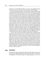
wavelength of the light signal. A basic understanding of light propagation in these
fibers can be obtained using the so-called geometrical optics model, illustrated in
Figure 1.16. In this model, a light ray bounces back and forth in the core, being
reflected at the core-cladding interface. The signal consists of multiple light rays,
each of which potentially takes a different path through the fiber. Each of these
different paths corresponds to a
propagation mode.
The length of the different paths
is different, as seen in the figure. Each mode therefore travels with a slightly different
speed compared to the other modes.
The other key devices needed for optical fiber transmission are light sources
and receivers. Compact semiconductor lasers and light-emitting diodes (LEDs) pro-
vided practical light sources. These lasers and LEDs were simply turned on and off
rapidly to transmit digital (binary) data. Semiconductor photodetectors enabled the
conversion of the light signal back into the electrical domain.
The early telecommunication systems (late 1970s through the early 1980s) used
multimode fibers along with LEDs or laser transmitters in the 0.8 and 1.3/~m wave-
length bands. LEDs were relatively low-power devices that emitted light over a fairly
wide spectrum of several nanometers to tens of nanometers. A laser provided higher
output power than an LED and therefore allowed transmission over greater dis-
tances before regeneration. The early lasers were

multilongitudinal mode
(MLM)
Fabry-Perot lasers. These MLM lasers emit light over a fairly wide spectrum of
several nanometers to tens of nanometers. The actual spectrum consists of multiple
spectral lines, which can be thought of as different longitudinal modes, hence the
1.8 Network Evolution 35
Figure 1.16 Geometrical optics model to illustrate the propagation of light in an optical
fiber. (a) Cross section of an optical fiber. The fiber has an inner core and an outer cladding,
with the core having a slightly higher refractive index than the cladding. (b) Longitudinal
view. Light rays within the core hitting the core-cladding boundary are reflected back
into the core by total internal reflection.
term MLM. Note that these longitudinal laser modes are different from the propa-
gation modes inside the optical fiber! While both LEDs and MLM lasers emit light
over a broad spectrum, the spectrum of an LED is continuous, whereas the spectrum
of an MLM laser consists of many periodic lines.
These early systems had to have regenerators every few kilometers to regenerate
the signal. Regenerators were expensive devices and continue to be expensive today,
so it is highly desirable to maximize the distance between regenerators. In this case,
the distance limitation was primarily due to a phenomenon known as
intermodal
dispersion.
As we saw earlier, in a multimode fiber, the energy in a pulse travels in dif-
ferent modes, each with a different speed. At the end of the fiber, the different modes
arrive at slightly different times, resulting in a smearing of the pulse. This smearing
in general is called
dispersion,
and this specific form is called intermodal dispersion.
Typically, these early systems operated at bit rates ranging from 32 to 140 Mb/s
with regenerators every 10 km. Such systems are still used for low-cost computer
interconnection at a few hundred megabits per second over a few kilometers.

1.8.2
Single-Mode Fiber
The next generation of systems deployed starting around 1984 used
single-mode
fiber as a means of eliminating intermodal dispersion, along with MLM Fabry-Perot
lasers in the 1.3 #m wavelength band. Single-mode fiber has a relatively small core
diameter of about 8 to 10 #m, which is a small multiple of the operating wavelength
36
INTRODUCTION TO OPTICAL NETWORKS
range of the light signal. This forces all the energy in a light signal to travel in the
form of a single mode. Using single-mode fiber effectively eliminated intermodal
dispersion and enabled a dramatic increase in the bit rates and distances possible
between regenerators. These systems typically had regenerator spacings of about
40 km and operated at bit rates of a few hundred megabits per second. At this point,
the distance between regenerators was limited primarily by the fiber loss.
The next step in this evolution in the late 1980s was to deploy systems in the
1.55 t~m wavelength window to take advantage of the lower loss in this window,
relative to the 1.3/zm window. This enabled longer spans between regenerators. At
this point, another impairment, namely,
chromatic dispersion,
started becoming a
limiting factor as far as increasing the bit rates was concerned. Chromatic dispersion
is another form of dispersion in optical fiber (we looked at intermodal dispersion
earlier). As we saw in Section 1.7, the energy in a light signal or pulse has a finite
bandwidth. Even in a single-mode fiber, the different frequency components of a pulse
propagate with different speeds. This is due to the fundamental physical properties
of the glass. This effect again causes a smearing of the pulse at the output, just as with
intermodal dispersion. The wider the spectrum of the pulse, the more the smearing
due to chromatic dispersion. The chromatic dispersion in an optical fiber depends on
the wavelength of the signal. It turns out that without any special effort, the standard

silica-based optical fiber has essentially no chromatic dispersion in the 1.3/~m band,
but has significant dispersion in the 1.55/zm band. Thus chromatic dispersion was
not an issue in the earlier systems at 1.3/zm.
The high chromatic dispersion at 1.55/zm motivated the development of
dispersion-shifted fiber.
Dispersion-shifted fiber is carefully designed to have zero
dispersion in the 1.55/zm wavelength window so that we need not worry about
chromatic dispersion in this window. However, by this time there was already a large
installed base of standard single-mode fiber deployed for which this solution could
not be applied. Some carriers, particularly NTT in Japan and MCI (now part of
Worldcom) in the United States, did deploy dispersion-shifted fiber.
At this time, researchers started looking for ways to overcome chromatic disper-
sion while still continuing to make use of standard fiber. The main technique that
came into play was to reduce the width of the spectrum of the transmitted pulse.
As we saw earlier, the wider the spectrum of the transmitted pulse, the greater the
smearing due to chromatic dispersion. The bandwidth of the transmitted pulse is at
least equal to its modulation bandwidth. On top of this, however, the bandwidth
may be determined entirely by the width of the spectrum of the transmitter used.
The MLM Fabry-Perot lasers, as we said earlier, emitted over a fairly wide spectrum
of several nanometers (or, equivalently, hundreds of gigahertz), which is much larger
than the modulation bandwidth of the signal itself. If we reduce the spectrum of the
transmitted pulse to something close to its modulation bandwidth, the penalty due
1.8 Network Evolution 37
1.8.3
to chromatic dispersion is significantly reduced. This motivated the development of
a laser source with a narrow spectral widthmthe
distributed-feedback
(DFB) laser.
A DFB laser is an example of a
single-longitudinal mode

(SLM) laser. An SLM
laser emits a narrow single-wavelength signal in a single spectral line, in contrast
to MLM lasers whose spectrum consists of many spectral lines. This technological
breakthrough spurred further increases in the bit rate to more than 1 Gb/s.
Optical Amplifiers and WDM
The next major milestone in the evolution of optical fiber transmission systems was
the development of
erbium-doped fiber amplifiers
(EDFAs) in the late 1980s and early
1990s. The EDFA basically consists of a length of optical fiber, typically a few meters
to tens of meters, doped with the rare earth element erbium. The erbium atoms in the
fiber are
pumped
from their ground state to an excited state at a higher energy level
using a pump source. An incoming signal photon triggers these atoms to come down
to their ground state. In the process, each atom emits a photon. Thus incoming signal
photons trigger the emission of additional photons, resulting in optical amplification.
Due to a unique coincidence of nature, the difference in energy levels of the atomic
states of erbium line up with the 1.5 #m low-loss window in the optical fiber. The
pumping itself is done using a pump laser at a lower wavelength than the signal
because photons with a lower wavelength have higher energies and energy can be
transferred only from a photon of higher energy to that with a lower energy. The
EDFA concept was invented in the 1960s but had to wait for the availability of
reliable high-power semiconductor pump lasers in the late 1980s and early 1990s
before becoming commercially viable.
EDFAs spurred the deployment of a completely new generation of systems. A
major advantage of EDFAs is that they are capable of amplifying signals at many
wavelengths simultaneously. This provided another way of increasing the system
capacity: rather than increasing the bit rate, keep the bit rate the same and use more
than one wavelength; that is, use wavelength division multiplexing. EDFAs were

perhaps the single biggest catalyst aiding the deployment of WDM systems. The use
of WDM and EDFAs dramatically brought down the cost of long-haul transmission
systems and increased their capacity. At each regenerator location, a single optical
amplifier could replace an entire array of expensive regenerators, one per fiber.
This proved to be so compelling that almost every long-haul carrier has widely
deployed amplified WDM systems today. Moreover WDM provided the ability to
turn on capacity quickly, as opposed to the months to years it could take to deploy
new fiber. WDM systems with EDFAs were deployed starting in the mid-1990s and
are today achieving capacities over 1 Tb/s over a single fiber. At the same time,
transmission bit rates on a single channel have risen to 10 Gb/s. Among the earliest
38 INTRODUCTION TO OPTICAL NETWORKS
WDM systems deployed were AT&T's 4-wavelength long-haul system in
1995
and
IBM's 20-wavelength MuxMaster metropolitan system in
1994.
With the advent of EDFAs, chromatic dispersion again reared its ugly head. In-
stead of regenerating the signal every 40 to 80 km, signals were now transmitted
over much longer distances because of EDFAs, leading to significantly higher pulse
smearing due to chromatic dispersion. Again, researchers found several techniques to
deal with chromatic dispersion. The transmitted spectrum could be reduced further
by using an external device to turn the laser on and off (called
external modula-
tion),
instead of directly turning the laser on and off (called
direct modulation).
Using external modulators along with DFB lasers and EDFAs allowed systems to
achieve distances of about 600 km at 2.5 Gb/s between regenerators over standard
single-mode fiber at
1.55/~m.

This number is substantially less at 10 Gb/s.
The next logical invention was to develop
chromatic dispersion compensation
techniques. A variety of chromatic dispersion compensators were developed to com-
pensate for the dispersion introduced by the fiber, allowing the overall residual dis-
persion to be reduced to within manageable limits. These techniques have enabled
commercial systems to achieve distances of several thousand kilometers between
regenerators at bit rates as high as 10 Gb/s per channel.
At the same time, several other impairments that were second- or third-order
effects earlier began to emerge as first-order effects. Today, this list includes nonlinear
effects in fiber, the nonflat gain spectrum of EDFAs, and various polarization-related
effects. There are several types of nonlinear effects that occur in optical fiber. One
of them is called
four-wave mixing
(FWM). In FWM, three light signals at different
wavelengths interact in the fiber to create a fourth light signal at a wavelength that
may overlap with one of the light signals. As we can imagine, this signal interferes
with the actual data that is being transmitted on that wavelength. It turns out
paradoxically that the higher the chromatic dispersion, the lower the effect of fiber
nonlinearities. Chromatic dispersion causes the light signals at different wavelengths
to propagate at different speeds in the fiber. This in turn causes less overlap between
these signals, as the signals go in and out of phase with each other, reducing the effect
of the FWM nonlinearity.
The realization of this trade-off between chromatic dispersion and fiber nonlin-
earities stimulated the development of a variety of new types of single-mode fibers
to manage the interaction between these two effects. These fibers are tailored to pro-
vide less chromatic dispersion than conventional fiber but, at the same time, reduce
nonlinearities. We devote Chapter 5 to the study of these impairments and how they
can be overcome; we discuss the origin of many of these effects in Chapter 2.
Today we are seeing the development of high-capacity amplified terabits/second

WDM systems with hundreds of channels at 10 Gb/s, with channel spacings as low as
50 GHz, with distances between electrical regenerators extending to a few thousand
1.8 Network Evolution
39
Table
1.2 Different wavelength bands in optical fiber. The
ranges are approximate and have not yet been standardized.
Band Descriptor
Wavelength range
(nm)
O-band Original 1260 to 1360
E-band Extended 1360 to 1460
S-band Short 1460 to 1530
C-band Conventional 1530 to 1565
L-band Long 1565 to 1625
U-band Ultra-long 1625 to 1675
kilometers. Systems operating at 40 Gb/s channel rates are in the research laborato-
ries, and no doubt we will see them become commercially available soon. Meanwhile,
recent experiments have achieved terabit/second capacities and stretched the distance
between regenerators to several thousand kilometers [Cai01, Bak01, VPM01], or
achieved total capacities of over 10 Tb/s [Fuk01, Big01] over shorter distances.
Table 1.2 shows the different bands available for transmission in single-mode
optical fiber. The early WDM systems used the C-band, primarily because that was
where EDFAs existed. Today we have EDFAs that work in the L-band, which allow
WDM systems to use both the C- and L-bands. We are also seeing the use of other
types of amplification (such as Raman amplification, a topic that we will cover in
Chapter 3) that complement EDFAs and hold the promise to open up other fiber
bands such as the S-band and the U-band for WDM applications. Meanwhile, the
development of new fiber types is also opening up a new window in the so-called
E-band. This band was previously not feasible due to the high fiber loss in this

wavelength range. New fibers have now been developed that reduce the loss in this
range. However, there are still no good amplifiers in this band, so the E-band is useful
mostly for short-distance applications.
1.8.4
Beyond Transmission Links to Networks
The late 1980s also witnessed the emergence of a variety of first-generation op-
tical networks. In the data communications world, we saw the deployment of
metropolitan-area networks, such as the 100 Mb/s fiber distributed data interface
(FDDI), and networks to interconnect mainframe computers, such as the 200 Mb/s
enterprise serial connection (ESCON). Today we are seeing the proliferation of stor-
age networks using the 1 Gb/s Fibre Channel standard for similar applications. In
the telecommunications world, standardization and mass deployment of SONET in
North America and the similar SDH network in Europe and Japan began. All these