Optical Networks: A Practical Perspective - Part 50 pot

460
WDM NETWORK DESIGN
t, l, r,
i ~ r2
,2 I "i
t4 ~ ~ r4
9
I
I
I
i'I
I
i
I
i
t 5 i r 5
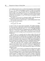
Figure 8.13 An example to illustrate the difference between having and not having
wavelength conversion.
L lightpaths use this link, L wavelengths will clearly be sufficient to accommodate
this request. However, without wavelength conversion, the number of wavelengths
required could be much larger. The important question is, How much larger? We
will study this problem in detail in Section 8.5, under various conditions, but we
consider one (somewhat extreme) example now.
Example 8.6 Consider the network shown in Figure 8.13. The set of lightpath
requests is shown in the figure to be the following. Transmitter
ti
must be con-
nected to receiver
rN-i+l,
where N is the number of transmitters or receivers.
Clearly, there are many routes for each lightpath. Interestingly, however, regard-

less of how we route each lightpath, any two lightpaths belonging to this set
of requests must share a common link. Thus each lightpath must be assigned
a different wavelength, requiring a total of N wavelengths to satisfy this set of
requests.
If we are clever about how we route these lightpaths, we can arrange matters
so that at most two lightpaths use a given link, as shown in the figure. This
means that the load is 2. Thus two wavelengths are sufficient to satisfy this set of
requests if full wavelength conversion is available at each node in the network.
Does this mean that full wavelength conversion is absolutely needed? Luckily for
us, the example shown here is a worst-case scenario. We will quantify the benefit
due to wavelength conversion in Section 8.5.
8.2 LTD and RWA Problems
461
8.2.4
Relationship to Graph Coloring
It turns out that the WA problem described earlier is closely related to the problem
of coloring the nodes in a graph. To understand this better, consider a graph repre-
sentation of the network G, where the vertices of the graph represent nodes in the
network, with an undirected edge between two vertices corresponding to an optical
fiber link between the corresponding nodes. Figure 8.14(a) is an example. The route
for each lightpath corresponds to a path in G, and thus the set of routes that have
been specified for the lightpaths corresponds to a set of paths, say, P. Now consider
another graph, the
path graph
of G, denoted by
P (G),
which is constructed as fol-
lows. Each path in G corresponds to a node in
P (G),
and two nodes in

P(G)
are
connected by an (undirected) edge if the corresponding paths in P share a common
edge in G. Figure 8.14(b) shows the path graph of the graph in Figure 8.14(a).
Solving the WA problem is then equivalent to solving the classical graph coloring
problem on P(G); that is, we have to assign a color to each node of
P(G)
such
that adjacent nodes are assigned distinct colors and the total number of colors is
minimized. These colors correspond to wavelengths used on the paths in G. The
minimum number of colors needed to color the nodes of a graph in this manner is
called the
chromatic number
of the graph. Thus the minimum number of wavelengths
required to solve the WA problem is the chromatic number of P(G).
Example 8.7 Let the graph G depicting the network be as shown in Fig-
ure 8.14. Since there is only one path between any pair of nodes in G, given the
set of node pairs to be connected by lightpaths, the routes are uniquely deter-
mined. So we have only to solve the WA problem. Suppose we need to set up
lightpaths between nodes 1 and 2, 2 and 3, and 1 and 3. The resulting path graph,
P(G),
is also shown in the same figure. The chromatic number of
P(G)
is 3, and
a coloring of
P(G)
in three colors is also shown. Thus we need three wavelengths
to solve the WA problem in this example.
Coloring an arbitrary graph is a hard problem that has been intensively studied
for several decades. In fact, it is an example of a class of problems, called

NP-complete
problems [GJ79], which are considered to be hard to solve. However, there are several
special classes of graphs for which fast coloring algorithms have been found. If the
P (G) we are interested in belongs to one of these special classes, then we can find an
exact solution to the WA problem. Otherwise, unless P (G) has only a few nodes, we
have to content ourselves with finding an approximate solution to the WA problem.
Many fast but approximate (heuristic) algorithms have been devised for the general
graph coloring problem (see, for example, [Big90, dW90]), and these algorithms can
be used to find good but approximate solutions to the WA problem.
462
WDM NETWORK DESIGN
Figure 8.14 Illustrating the relationship to graph coloring.
Although this transformation illustrates the relationship to graph coloring, it
does not prove that the WA problem is in itself hard or, specifically, NP-complete.
To show this, you need to perform the transformation in the opposite direction,
namely, take an instance of a graph coloring problem and convert it into an instance
of the WA problem. This has been done in [CGK92], which proves that WA is indeed
NP-complete. However, it is still possible to obtain useful bounds for this problem,
as well as develop algorithms for several specific and important topologies such as
ring networks, as we will see next.
8.3
Dimensioning Wavelength-Routing Networks
The key aspect of designing a wavelength-routing network is determining the number
and, more generally, the set of wavelengths that must be provided on each WDM
link. We call this the
wavelength dimensioning problem.
In most practical situations today, the network is designed to support a certain,
fixed traffic matrix. The traffic matrix may be in terms of lightpaths or in terms
of higher-layer (IP, SONET) traffic. In the former case, only the RWA needs to be
solved, while in the latter case, both the LTD and RWA problems must be solved (in

conjunction or separately). By and large, this is the approach used in practice today to
design wavelength-routing networks. The solution of the RWA problem determines
the specific set of wavelengths that must be provided on each link to realize the
required lightpath topology, and thus solves the dimensioning problem. This is the
offline
RWA problem since we are given all the lightpaths at once, and is useful in
the network planning stage. Once a network is operational, the RWA problem has
to be solved for one lightpath at a time, when the lightpath is required to be set up.
This is the
online
RWA problem. With the reduction in lightpath service provisioning
8.3 Dimensioning Wavelength-Routing Networks 463
Figure
8.15 The three-node network of Figure 8.1(c) with the static OADM at the
central node replaced by a reconfigurable OADM, or OXC. The OXC allows the
set of lightpaths added/dropped at the node to be decided dynamically based on the
lightpath/traffic requirements.
times that is being faced by carriers, it is becoming increasingly important to find
good, rapid solutions to the online RWA problem.
While the specific sets of wavelengths obtained by solving the offline RWA prob-
lem can be provisioned in a network without OXCs, OXCs are used where flexibility
in handling different traffic matrices is needed. Without OXCs, the lightpaths must
be established by a static, or a priori, mapping of incoming wavelengths to outgoing
wavelengths at each node. Since most of the wavelength-routing networks that have
been deployed today do not use OXCs, the lightpaths have been established in such
a static fashion in these networks. When OXCs are deployed, by appropriate config-
uration of the OXCs, the optical layer can change the lightpath topology and hence
adapt to different traffic requirements. Thus this approach can support any one of
several different lightpath topologies, and consequently, traffic requirements at the
higher layer, on the same fiber topology with the same optical layer equipment. Since

the higher-layer traffic requirements are usually unknown, this flexibility is quite
important in building a future-proof optical network.
Example
8.8 To illustrate the flexibility obtained by using OXCs in the net-
work, consider the three-node linear network example again. By replacing the
static OADM in Figure 8.1(c) by a reconfigurable OADM, or OXC, with 30
ports, we obtain the node design shown in Figure 8.15. This design can han-
dle any combination of traffic that does not require termination of more than
100 Gb/s of traffic at each node, in contrast to the design of Figure 8.1(c), which
was designed for a specific traffic matrix: 50 Gb/s of traffic between each pair of
nodes.
Solving the dimensioning problem determines not only the number of wave-
lengths that need to be supported on each link, but also determines the sizes of the
OLTs and the OXCs. The size of the OXC also depends on the maximum number of
464
WDM NETWORK DESIGN
lightpaths to be terminated at each node, which corresponds to the number of router
interface cards provided at that node.
As discussed above, in contemporary practice, the design of wavelength-routing
networks today is accomplished by forecasting a certain fixed traffic matrix between
the nodes. This forecast is revised every six months or so, and based on this forecast,
the network is upgraded with the addition of more capacities on the WDM links, or
more links, or additional nodes, or a combination of these approaches. Solving the
network upgrade problem is similar to solving the original problem, except that the
lightpaths that have already been established are usually not disturbed.
We can view the above approach of forecasting a fixed traffic matrix and di-
mensioning the network to support the forecasted traffic as using a "deterministic"
traffic model since the variations in traffic are not explicitly accounted for during the
design phase, though the use of crossconnects in the network enables some of these
variations to be handled at the time of actually setting up the lightpaths. Another

approach to capacity planning is through the use of statistical traffic models, which
we will discuss in Section 8.4.
In a wavelength-routing network, if the nodes have full conversion capability, the
situation is the same as in classical circuit-switched telephone networks: a lightpath
is equivalent to a phone call and must be assigned one circuit on each of the links it
traverses. Another approach studied extensively by researchers is to dimension opti-
cal networks with no or limited conversion capabilities, to support the same traffic
that would be supported using full conversion within the optical layer. We discuss
these methods in Section 8.5. In this case, as well as in the case of statistical models,
we consider only the RWA problem and not the LTD problem. Thus, grooming issues
that are part of the LTD problem are not discussed. The problem of determining the
location of regenerators is also outside the scope of our discussion.
8.4
Statistical Dimensioning Models
There are two classes of statistical traffic models that can be used in solving the
dimensioning problem. These models differ in their assumptions regarding what is
known about the set or sets of lightpaths that must be supported. In some cases,
these models also assume that each link supports the same number (and set) of
wavelengths, but this may not always be appropriate.
1. First-passage model: In this model, the network is assumed to start with no
lightpaths at all. Lightpaths arrive randomly according to a statistical model and
8.4 Statistical Dimensioning Models
465
have to be set up on the optical layer. Some lightpaths may depart as well, but it
is assumed that, on average, the number of lightpaths will keep increasing and
eventually we will have to reject a lightpath request. (Thus the rate of arrival of
lightpath requests exceeds the rate of termination of lightpaths, and the network
is not in equilibrium.) We are interested in dimensioning the WDM links so
that the first lightpath request rejection will occur, with high probability, after a
specified period of time, T. This is a reasonable model today since lightpaths are

long lived. This longevity, combined with the cost of a high-bandwidth lightpath
today, means that network operators are unlikely to reject a lightpath request.
Rather, they would like to upgrade their network by the addition of more capacity
on existing links, or by the addition of more links, in order to accommodate the
lightpath request. The time period T corresponds approximately to the time by
which the operators must institute such upgrades in order to avoid rejecting
lightpath requests.
2. Blocking model: In this model, the lightpath requests are treated in the same
way that a telephone network treats phone calls. Requests are assumed to arrive
and depart at random instants according to a statistical model. (However, the
network is assumed to be in equilibrium, that is, the rate of arrival and the rate
of termination of lightpaths are equal.) The assumption is that most requests
must be honored but occasionally requests may be blocked. The goal again is to
dimension the WDM links so that the blocking events are relatively rare (say, a
fraction of 1%). This is a futuristic model since lightpaths today are relatively
long lived, but it is quite possible that lightpaths will be provided on demand
by some operators in the future. In such a scenario, this would be a reasonable
model to use in order to dimension the WDM links.
For these statistical models, the
analysis problem
is easier to solve than the
design
problem.
For example, in the blocking model, it is easier to calculate the blocking
probabilities on each of the links given the link capacities (and the traffic model)
than it is to design the link capacities to achieve prespecified blocking probabilities.
Similarly, in the first-passage model, it is easier to calculate the (statistics of the)
first time at which the network operator will have to block a lightpath request for
given link capacities than it is to design the link capacities to achieve a prespeci-
fled first-passage time. However, the capacity design or dimensioning problem can

be solved by iterating on the analysis problem. For example, we can calculate the
blocking probabilities for a given set of capacities, and if the blocking is not accept-
able on some links, increase the capacities of those links and recalculate the blocking
probabilities. In the rest of this section, we will address the analysis problems.
466
WDM NETWORK DESIGN
96
5~ 88
'qF
92
I
Figure 8.16 A
20-node, 32-1ink network representing a skeleton of the ARPANET. An average
of one lightpath request is assumed to arrive every month, between every pair of nodes, and this
lightpath is assumed to be in place for an average of one year. The link capacities shown are calculated
such that no link will need a capacity upgrade within two years, with high (85%) probability.
8.4.1
First-Passage Model
In this model, the network is assumed to start with no lightpaths, but the link
capacities are given. The model is analytically tractable only if we assume that
lightpath requests follow a Poisson process and their durations are exponentially
distributed. (This is the standard assumption in telephone networks for the statistics
of phone calls. Thus, this is tantamount to assuming that lightpath requests are like
phone calls.) The network can be modeled by a Markov chain where the state of
the Markov chain represents the set of calls in progress. You can consider both fully
wavelength-converting crossconnects and OXCs with no conversion capability. The
Markov chain approach is somewhat tractable only in the case of full wavelength
conversion. An approximate analysis of this model appears in [NS02].
We do not describe the mathematical details of the ana!ytical model that can be
found in INS02], but we present the outcome of such an analysis for a moderate-sized

network. The network considered is shown in Figure 8.16. It has 20 nodes and 32
links and represents a skeleton of the original ARPANET. The request for lightpaths
on each of the possible 190 routes is assumed to arrive at a rate of one request per
month (but with a Poisson distribution). The average lightpath lease time is assumed
to be one year (with an exponential distribution). It is assumed that the capacity on
each link can be a multiple of four wavelengths. The capacities of the links shown in
Figure 8.16 are determined such that the probability that any of these links needs a
capacity upgrade within two years is less than 15%.
8.4 Statistical Dimensioning Models 467
8.4.2
Blocking Model
In this model, we assume that lightpath arrival and termination requests follow a
statistical pattern. We may allow some lightpath requests to be blocked and are
interested therefore in minimizing the blocking probability. In this case, a measure
of the lightpath traffic is the
offered load,
which is defined as the arrival rate of
lightpath requests multiplied by the average lightpath duration.
In practice, the maximum blocking probability is specified, say, 1%. We are then
interested in determining the maximum offered load that the network can support.
A more convenient metric is the wavelength
reuse factor, R,
which we define as the
offered load per wavelength in the network that can be supported with the specified
blocking probability. Clearly, R could depend on (1) the network topology, (2) the
traffic distribution in the network, (3) the actual RWA algorithm used, and (4) the
number of wavelengths available.
In principle, ifwe are given (1)-(4), we can determine the reuse factor R. However,
this problem is difficult to solve analytically for specific RWA algorithms. When the
routes between the source-destination nodes in the network are fixed (fixed routing)

and an available wavelength is chosen randomly, the blocking probabilities (and
hence the reuse factor) can be analytically estimated for a reasonable number of
wavelengths (say, up to 64). A discussion of these analytical techniques is beyond the
scope of this book but can be found in [SS00]. The results of such an analysis can be
used to dimension the links for a given blocking probability just as in the case of the
first-passage model discussed above.
When the routing is not fixed, estimating the blocking probabilities or reuse
factors is analytically intractable, and in practice, the best way to estimate R even for
small networks is by simulation. It is possible to analytically calculate the maximum
value of R when the number of wavelengths is very large for small networks; this
has been done in [RS95] and serves as an upper bound on the reuse factor for
practical values of the number of wavelengths. When the number of wavelengths is
small, simulation techniques can be used to compute the reuse factor. To this end,
we summarize some of the simulation results from [RS95]. We will also compare the
simulation results with the analytically calculated upper bound on the reuse factor.
We will use randomly chosen graphs to model the network, assume a Poisson arrival
process with exponential holding times, assume a uniform traffic distribution, and
use the following RWA algorithm.
Algorithm 8.2
1. Number the W available wavelengths from 1 to W.
468
WDM NETWORK DESIGN
9 ii
Figure
8.17 Reuse factor plotted against the number of wavelengths for a 32-node
random graph with average degree 4, with full wavelength conversion and no wavelength
conversion, from [RS95]. The horizontal line indicates the value of the reuse factor that
can be achieved with an infinite number of wavelengths with full wavelength conversion,
which can be calculated analytically.
2. For a lightpath request between two nodes, assign to it the first available

wavelength on a fixed shortest path between the two nodes.
Figure 8.17 shows the reuse factor plotted against the number of wavelengths
for a 32-node random graph with average node degree 4. The figure also shows the
value of the blocking probability that can be achieved with an infinite number of
wavelengths, which can be calculated analytically as mentioned before [RS95]. The
reuse factor is slightly higher with full conversion. The interesting point to be noted
is that the reuse factor improves as the number of wavelengths increases. This is due
to a phenomenon known as
trunking efficiency,
which is familiar to designers of
telephone networks. Essentially, the blocking probability is reduced if you scale up
both traffic and link capacities by the same factor. To illustrate this phenomenon,
consider a single link with Poisson arrivals with offered load p with W wavelengths.
The blocking probability on this link is given by the famous Erlang-B formula:
Pb(P, W) =
pW
W~
pi "
8.4 Statistical Dimensioning Models 469
The reader can verify that if both the offered traffic and the number of wavelengths
are scaled by a factor c, > 1, then
Pb (~P, ~ W) < Pb (P, W)
and
Pb (otp, ol W) ~ 0 as o~ ~ ~ if
p
_~ W.
Figure 8.18 shows the reuse factor plotted against the number of nodes N. The
value of R for each N is obtained by averaging the simulated results over three
different random graphs, each of average degree 4. The figure shows that (1) R
increases with N, and (2) the difference between not having conversion and having

it also increases with N. Note that observation (1) is to be expected because the
average lightpath length (in number of hops) in the network grows as log N, whereas
the number of links in the network grows as N. Thus we would expect the reuse
factor to increase roughly as N/log N. The reason for observation (2) is that the
average path length (or hops) of a lightpath in the network increases with N. We will
see next that wavelength converters are more effective when the network has longer
paths.
A similar simulation has been performed in [KA96] for ring networks. In general,
the increase in reuse factor obtained after using wavelength conversion was found to
be very small. This may seem counterintuitive initially because hop lengths in rings
are quite large compared to mesh networks. We will see next that hop length alone
is not the sole criterion for determining the gain due to wavelength conversion. In
rings, lightpaths that overlap tend to do so over a relatively large number of links,
compared to mesh networks. We will see that the larger this overlap, the less the gain
due to wavelength conversion.
Factors Governing Wavelength Reuse
We will next quantify the impact of the number of hops and the "overlap" between
lightpaths on the wavelength conversion gain. We assume a statistical model for the
lightpath requests and make a highly simplified comparison of the probability that
a lightpath request will be denied (blocked) when the network uses wavelength con-
verters and when it does not, based on [BH96]. We assume that the route through the
network for each lightpath is specified. When the network does not use wavelength
converters, the wavelength assignment algorithm assigns an arbitrary but identical
wavelength on every link of the route when one such wavelength is free (not assigned
to any other lightpath) on every link of the path. When the network uses wavelength