Handbook of mathematics for engineers and scienteists part 44 pps

6.3. FUNCTIONS OF SEVERAL VARIABLES.PARTIAL DERIVATIVES 269
6.3.4. Extremal Points of Functions of Several Variables
6.3.4-1. Conditions of extremum of a function of two variables.
1
◦
. Points of minimum, maximum, or extremum. A point (x
0
, y
0
) is called a point of local
minimum (resp., maximum)ofafunctionz = f(x, y) if there is a neighborhood of (x
0
, y
0
)
in which the function is defined and satisfies the inequality f(x, y)>f (x
0
, y
0
) (resp.,
f(x, y)<f (x
0
, y
0
)). Points of maximum or minimum are called points of extremum.
2
◦
.Anecessary condition of extremum. If a function has the first partial derivatives at a
point of its extremum, these derivatives must vanish at that point. It follows that in order
to find points of extremum of such a function z = f(x, y), one should find solutions of the
system of equations

f
x
(x, y)=0, f
y
(x, y)=0.
The points whose coordinates satisfy this system are called stationary points. Any point of
extremum of a differentiable function is its stationary point, but not every stationary point
is a point of its extremum.
3
◦
. Sufficient conditions of extremum are used for the identification of points of extremum
among stationary points. Some conditions of this type are given below.
Suppose that the function z = f(x, y) has continuous second derivatives at a stationary
point. Let us calculate the value of the determinant at that point:
Δ = f
xx
f
yy
– f
2
xy
.
The following implications hold:
1)IfΔ > 0, f
xx
> 0, then the stationary point is a point of local minimum;
2)IfΔ > 0, f
xx
< 0, then the stationary point is a point of local maximum;
3)IfΔ < 0, then the stationary point cannot be a point of extremum.

In the degenerate case, Δ = 0, a more delicate analysis of a stationary point is required. In
this case, a stationary point may happen to be a point of extremum and maybe not.
Remark. In order to find points of extremum, one should check not only stationary points, but also points
at which the first derivatives do not exist or are infinite.
4
◦
. The smallest and the largest values of a function.Letf(x, y) be a continuous function
in a closed bounded domain D. Any such function takes its smallest and its largest values
in D.
If the function has partial derivatives in D, except at some points, then the follow-
ing method can be helpful for determining the coordinates of the points (x
min
, y
min
)and
(x
max
, y
max
) at which the function attains its minimum and maximum, respectively. One
should find all internal stationary points and all points at which the derivatives are infinite
or do not exist. Then one should calculate the values of the function at these points and
compare these with its values at the boundary points of the domain, and then choose the
largest and the smallest values.
6.3.4-2. Extremal points of functions of three variables.
For functions of three variables, points of extremum are defined in exactly the same way as
for functions of two variables. Let us briefly describe the scheme of finding extremal points
of a function u = Φ(x, y, z). Finding solutions of the system of equations
Φ
x

(x, y,z)=0, Φ
y
(x, y,z)=0, Φ
z
(x, y,z)=0,
270 LIMITS AND DERIVATIVES
we determine stationary points. For each stationary point, we calculate the values of
Δ
1
= Φ
xx
, Δ
2
=



Φ
xx
Φ
xy
Φ
xy
Φ
yy



, Δ
3

=





Φ
xx
Φ
xy
Φ
xz
Φ
xy
Φ
yy
Φ
yz
Φ
xz
Φ
yz
Φ
zz





.

The following implications hold:
1)IfΔ
1
> 0, Δ
2
> 0, Δ
3
> 0, then the stationary point is a point of local minimum;
2)IfΔ
1
< 0, Δ
2
> 0, Δ
3
< 0, then the stationary point is a point of local maximum.
6.3.4-3. Conditional extremum of a function of two variables. Lagrange function.
A point (x
0
, y
0
) is called a point of conditional or constrained minimum (resp., maximum)
of a function
z = f (x, y)(6.3.4.1)
under the additional condition*
ϕ(x, y)=0 (6.3.4.2)
if there is a neighborhood of the point (x
0
, y
0
)inwhichf (x, y)>f (x

0
, y
0
) (resp., f (x, y)<
f(x
0
, y
0
)) for all points (x, y) satisfying the condition (6.3.4.2).
For the determination of points of conditional extremum, it is common to use the
Lagrange function
Φ(x, y,λ)=f(x, y)+λϕ(x, y),
where λ is the so-called Lagrange multiplier. Solving the system of three equations (the
last equation coincides with the condition (6.3.4.2))
∂Φ
∂x
= 0,
∂Φ
∂y
= 0,
∂Φ
∂λ
= 0,
one finds stationary points of the Lagrange function (and also the value of the coefficient λ).
The stationary points may happen to be points of extremum. The above system yields
only necessary conditions of extremum, but these conditions may be insufficient; it may
happen that there is no extremum at some stationary points. However, with the help of other
properties of the function under consideration, it is often possible to establish the character
of a critical point.
Example 1. Let us find an extremum of the function

z = x
n
y,(6.3.4.3)
under the condition
x + y = a (a > 0, n > 0, x ≥ 0, y ≥ 0). (6.3.4.4)
Taking F (x, y)=x
n
y and ϕ(x, y)=x + y – a, we construct the Lagrange function
Φ(x, y, λ)=x
n
y + λ(x + y – a).
Solving the system of equations
Φ
x
≡ nx
n–1
y + λ = 0,
Φ
y
≡ x
n
+ λ = 0,
Φ
λ
≡ x + y – a = 0,
we find the coordinates of a unique stationary point,
x
◦
=
an

n + 1
, y
◦
=
a
n + 1
, λ
◦
=–

an
n + 1

n
,
which corresponds to the maximum of the given function, z
max
=
a
n+1
n
n
(n + 1)
n+1
.
* This condition is also called a constraint.
6.3. FUNCTIONS OF SEVERAL VARIABLES.PARTIAL DERIVATIVES 271
Remark. In order to find points of conditional extremum of functions of two variables, it is often convenient
to express the variable y through x (or vice versa) from the additional equation (6.3.4.2) and substitute the
resulting expression into the right-hand side of (6.3.4.1). In this way, the original problem is reduced to the

problem of extremum for a function of a single variable.
Example 2. Consider again the extremum problem of Example 1 for the function of two variables (6.3.4.3)
with the constraint(6.3.4.4). Afterthe eliminationof the variabley from (6.3.4.3)–(6.3.4.4), the original problem
is reduced to the extremum problem for the function z = x
n
(a – x) of one variable.
6.3.4-4. Conditional extremum of functions of several variables.
Consider a function u = f (x
1
, , x
n
)ofn variables under the condition that x
1
, , x
n
satisfy m equations (m < n):
⎧
⎪
⎪
⎨
⎪
⎪
⎩
ϕ
1
(x
1
, , x
n
)=0,

ϕ
2
(x
1
, , x
n
)=0,
,
ϕ
m
(x
1
, , x
n
)=0.
In order to find the values of x
1
, , x
n
for which f may have a conditional maximum or
minimum, one should construct the Lagrange function
Φ(x
1
, , x
n
; λ
1
, , λ
m
)=f + λ

1
ϕ
1
+ λ
2
ϕ
2
+ ···+ λ
m
ϕ
m
and equate to zero its first partial derivatives in the variables x
1
, , x
n
and the parameters
λ
1
, , λ
m
. From the resulting n + m equations, one finds x
1
, , x
n
(and also the values
of the unknown Lagrange multipliers λ
1
, , λ
m
). As in the case of functions of two

variables, the question whether the given function has points of conditional extremum can
be answered on the basis of additional investigation.
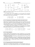
Example 3. Consider the problem of finding the shortest distance from the point (x
0
, y
0
, z
0
) to the plane
Ax + By + Cz + D = 0.(6.3.4.5)
The squared distance between the points (x
0
, y
0
, z
0
)and(x, y, z) is equal to
R
2
=(x – x
0
)
2
+(y – y
0
)
2
+(z – z
0
)

2
.(6.3.4.6)
In our case, the coordinates (x, y,z) should satisfy equation (6.3.4.5) (this point should belong to the plane).
Thus, our problem is to find the minimum of the expression (6.3.4.6) under the condition (6.3.4.5). The
Lagrange function has the form
Φ =(x – x
0
)
2
+(y – y
0
)
2
+(z – z
0
)
2
+ λ(Ax + By + Cz + D).
Equating to zero the derivatives of Φ in x, y, z, λ, we obtain the following system of algebraic equations:
2(x – x
0
)+Aλ = 0, 2(y – y
0
)+Bλ = 0, 2(z – z
0
)+Cλ = 0, Ax + By + Cz + D = 0.
Its solution has the form
x = x
0
–

1
2
Aλ, y = y
0
–
1
2
Bλ, z = z
0
–
1
2
Cλ, λ =
2(Ax
0
+ By
0
+ Cz
0
+ D)
A
2
+ B
2
+ C
2
.(6.3.4.7)
Thus we have a unique answer, and since the distance between a given point and the plane can be realized at a
single point (x, y, z), the values obtained should correspond to that distance. Substituting the values (6.3.4.7)
into (6.3.4.6), we find the squared distance

R
2
=
(Ax
0
+ By
0
+ Cz
0
+ D)
2
A
2
+ B
2
+ C
2
.
272 LIMITS AND DERIVATIVES
6.3.5. Differential Operators of the Field Theory
6.3.5-1. Hamilton’s operator and first-order differential operators.
The Hamilton’s operator or the nabla vector is the symbolic vector
∇ =

i
∂
∂x
+

j

∂
∂y
+

k
∂
∂z
.
This vector can be used for expressing the following differential operators:
1) gradient of a scalar function u(x, y, z):
grad u =

i
∂u
∂x
+

j
∂u
∂y
+

k
∂u
∂z
= ∇u;
2) divergence of a vector field a = P

i + Q


j + R

k:
diva =
∂P
∂x
+
∂Q
∂y
+
∂R
∂z
= ∇⋅a
(scalar product of the nabla vector and the vector a);
3) rotation of a vector field a = P

i + Q

j + R

k:
curla =







i


j

k
∂
∂x
∂
∂y
∂
∂z
PQR






= ∇ × a
(vector product of the nabla vector and the vector a).
Each scalar fi eld u(x, y, z) generates a vector field grad u. A vector field a(x, y,z)
generates two fields: the scalar field diva and the vector field curla.
6.3.5-2. Second-order differential operators.
The following differential identities hold:
1)curlgradu =

0 or (∇ × ∇) u =

0,
2)divcurla = 0 or ∇⋅(∇ × a)=0.
The following differential relations hold:

1)divgradu = Δu =
∂
2
u
∂x
2
+
∂
2
u
∂y
2
+
∂
2
u
∂z
2
,
2) curl curla =graddiva – Δa,
where Δ is the Laplace operator, Δu = ∇⋅(∇u)=∇
2
u.
References for Chapter 6
Adams, R., Calculus: A Complete Course, 6th Edition, Pearson Education, Toronto, 2006.
Boyer, C. B., The History of the Calculus and Its Conceptual Development, Dover Publications, New York,
1989.
Brannan, D., A First Course in Mathematical Analysis, Cambridge University Press, Cambridge, 2006.
Browder, A., Mathematical Analysis: An Introduction, Springer-Verlag, New York, 1996.
Courant, R. and John, F., Introduction to Calculus and Analysis, Vol. 1, Springer-Verlag, New York, 1999.

Edwards, C. H., and Penney, D., Calculus, 6th Edition, Pearson Education, Toronto, 2002.
Kline, M., Calculus: An Intuitive and Physical Approach, 2nd Edition, Dover Publications, New York, 1998.
Landau, E., Differential and Integral Calculus, American Mathematical Society, Providence, Rhode Island,
2001.
Silverman, R. A., Essential Calculus with Applications, Dover Publications, New York, 1989.
Zorich, V. A., Mathematical Analysis, Springer-Verlag, Berlin, 2004.
Chapter 7
Integrals
7.1. Indefinite Integral
7.1.1. Antiderivative. Indefinite Integral and Its Properties
7.1.1-1. Antiderivative.
An antiderivative (or primitive function) of a given function f(x)onaninterval(a, b)isa
differentiable function F (x) such that its derivative is equal to f(x)forallx (a, b):
F

(x)=f(x).
Example 1. Let f(x)=2x. Then the functions F (x)=x
2
and F
1
(x)=x
2
– 1 are antiderivatives of f(x),
since (x
2
)

= 2x and (x
2
– 1)


= 2x.
THEOREM.
Any function
f(x)
continuous on an interval
(a, b)
has infinitely many con-
tinuous antiderivatives on
(a, b)
.If
F (x)
is one of them, then any other antiderivative has
the form
F (x)+C
,where
C
is a constant.
7.1.1-2. Indefinite integral.
The indefinite integral of a function f(x)istheset,F (x)+C, of all its antiderivatives. This
fact is conventionally written as

f(x) dx = F (x)+C.
Here, f(x) is called the integrand (or the integrand function). The process of finding an
integral is called integration. The differential dx indicates that the integration is carried out
with respect to x.
Example 2.

6x
2

dx = 2x
3
+ C,since(2x
3
)

= 6x
2
.
7.1.1-3. Most important corollaries of the definition of the indefinite integral.
Differentiation is the inverse of integration:
d
dx


f(x) dx

= f (x).
Integration is the inverse of differentiation:*

f

(x) dx = f (x)+C.
The latter formula serves to make up tables of indefinite integrals. The procedure is
often reverse here: an integral is first given in explicit form (i.e., the function f(x)onthe
right-hand side is prescribed), and then the integrand is obtained by differentiation.
* Integration recovers the function from its derivative, to an additive constant.
273
274 INTEGRALS
7.1.2. Table of Basic Integrals. Properties of the Indefinite Integral.

Integration Examples
7.1.2-1. Table of basic integrals.
Listed below are most common indefinite integrals, which are important for the integration
of more complicated expressions:

x
a
dx =
x
a+1
a + 1
+ C (a ≠ –1),

dx
x
=ln|x| + C,

dx
x
2
+ a
2
=
1
a
arctan
x
a
+ C,


dx
x
2
– a
2
=
1
2a
ln



x – a
x + a



+ C,

dx
√
a
2
– x
2
=arcsin
x
a
+ C,


dx
√
x
2
+ a
=ln


x +
√
x
2
+ a


+ C,

e
x
dx = e
x
+ C,

a
x
dx =
a
x
ln a
+ C,


ln xdx = x ln x – x + C,

ln ax dx = x ln ax – x + C,

sin xdx =–cosx + C,

cos xdx=sinx + C,

tan xdx=–ln|cos x| + C,

cot xdx=ln|sin x| + C,

dx
sin x
=ln



tan
x
2



+ C,

dx
cos x
=ln




tan

x
2
+
π
4




+ C,

dx
sin
2
x
=–cotx + C,

dx
cos
2
x
=tanx + C,

arcsin xdx= x arcsin x +
√

1 – x
2
+ C,

arccos xdx= x arccos x –
√
1 – x
2
+ C,

arctan xdx= x arctan x –
1
2
ln(1 + x
2
)+C,

arccot xdx= x arccot x +
1
2
ln(1 + x
2
)+C,

sinh xdx=coshx + C,

cosh xdx=sinhx + C,

tanh xdx=lncoshx + C,


coth xdx=ln|sinh x| + C,

dx
sinh x
=ln



tanh
x
2



+ C,

dx
cosh x
= 2 arctan e
x
+ C,

dx
sinh
2
x
=–cothx + C,

dx
cosh

2
x
=tanhx + C,

arcsinh xdx= x arcsinh x –
√
1 + x
2
+ C,

arccosh xdx= x arccosh x –
√
x
2
– 1 + C,

arctanh xdx= x arctanh x +
1
2
ln(1 – x
2
)+C,

arccoth xdx= x arccoth x +
1
2
ln(x
2
– 1)+C,
where C is an arbitrary constant.


A more extensive table of indefinite integrals can be found in Section T2.1.
7.1.2-2. Properties of the indefinite integral.
1. A constant factor can be taken outside the integral sign:

af(x) dx = a

f(x) dx (a = const).
7.1. INDEFINITE INTEGRAL 275
2. Integral of the sum or difference of functions (additivity):

[f(x)
g(x)] dx =

f(x) dx

g(x) dx.
3. Integration by parts:

f(x)g

(x) dx = f(x)g(x)–

f

(x)g(x) dx.
4. Repeated integration by parts (generalization of the previous formula):

f(x)g
(n+1)

(x) dx = f(x)g
(n)
(x)–f

(x)g
(n–1)
(x)+···+(–1)
n
f
(n)
(x)g(x)
+(–1)
n+1

f
(n+1)
(x)g(x) dx, n = 0, 1,
5. Change of variable (integration by substitution):

f(x) dx =

f(ϕ(t)) ϕ

t
(t) dt, x = ϕ(t).
On computing the integral using the change of variable x = ϕ(t), one should rewrite the
resulting expression in terms of the original variable x using the back substitution t = ϕ
–1
(x).
7.1.2-3. Examples of direct integration of elementary functions.

1
◦
. With simple algebraic manipulation and the properties listed in Paragraph 7.1.2-2, the
integration may often be reduced to tabulated integrals.
Example 1.

2x – 1
√
x
dx =


2
√
x –
1
√
x

dx = 2

x
1/2
dx –

x
–1/2
dx =
4
3

x
3/2
– 2x
1/2
+ C.
2
◦
. Tabulated integrals can also be used where any function ϕ(x) appears in place of x;for
example,

e
x
dx = e
x
+ C =⇒

e
ϕ(x)
dϕ(x)=e
ϕ(x)
+ C;

dx
x
=ln|x| + C =⇒

d sin x
sin x
=ln|sin x| + C.
The reduction of an integral to a tabulated one may often be achieved by taking some

function inside the differential sign.
Example 2.

tan xdx=

sin xdx
cos x
=

–d cos x
cos x
=–

d cos x
cos x
=–ln|cos x| + C.
3
◦
. Integrals of the form

dx
ax
2
+ bx + c
,

dx
√
ax
2

+ bx + c
can be computed by making
a perfect square:
ax
2
+ bx + c = a

x +
b
2a

2
–
b
2
4a
+ c.
Then one should replace dx with the equal differential d

x +
b
2a

and use one of the four
formulas in the second and third rows in the table of integrals given in Paragraph 7.1.2-1.