Handbook of mathematics for engineers and scienteists part 144 pps
Bạn đang xem bản rút gọn của tài liệu. Xem và tải ngay bản đầy đủ của tài liệu tại đây (409.74 KB, 7 trang )
18.13. ELLIPTIC INTEGRALS 969
18.13. Elliptic Integrals
18.13.1. Complete Elliptic Integrals
18.13.1-1. Definitions. Properties. Conversion formulas.
Complete elliptic integral of the first kind:
K(k)=
π/2
0
dα
√
1 – k
2
sin
2
α
=
1
0
dx
(1 – x
2
)(1 – k
2
x
2
)
.
Complete elliptic integral of the second kind:
E(k)=
π/2
0
√
1 – k
2
sin
2
αdα=
1
0
√
1 – k
2
x
2
√
1 – x
2
dx.
The argument k is called the elliptic modulus (k
2
< 1).
Notation:
k
=
√
1 – k
2
, K
(k)=K(k
), E
(k)=E(k
),
where k
is the complementary modulus.
Properties:
K(–k)=K(k), E(–k)=E(k);
K(k)=K
(k
), E(k)=E
(k
);
E(k) K
(k)+E
(k) K(k)–K(k) K
(k)=
π
2
.
Conversion formulas for complete elliptic integrals:
K
1 – k
1 + k
=
1 + k
2
K(k),
E
1 – k
1 + k
=
1
1 + k
E(k)+k
K(k)
,
K
2
√
k
1 + k
=(1 + k) K(k),
E
2
√
k
1 + k
=
1
1 + k
2 E(k)–(k
)
2
K(k)
.
18.13.1-2. Representation of complete elliptic integrals in series form.
Representation of complete elliptic integrals in the form of series in powers of the modulus k:
K(k)=
π
2
1 +
1
2
2
k
2
+
1×3
2×4
2
k
4
+ ···+
(2n – 1)!!
(2n)!!
2
k
2n
+ ···
,
E(k)=
π
2
1 –
1
2
2
k
2
1
–
1×3
2×4
2
k
4
3
– ···–
(2n – 1)!!
(2n)!!
2
k
2n
2n – 1
– ···
.
970 SPECIAL FUNCTIONS AND THEIR PROPERTIES
Representation of complete elliptic integrals in the form of series in powers of the comple-
mentary modulus k
=
√
1 – k
2
:
K(k)=
π
1 +k
1 +
1
2
2
1 –k
1 +k
2
+
1×3
2×4
2
1 –k
1 +k
4
+ ···+
(2n –1)!!
(2n)!!
2
1 –k
1 +k
2n
+ ···
,
K(k)=ln
4
k
+
1
2
2
ln
4
k
–
2
1×2
(k
)
2
+
1×3
2×4
2
ln
4
k
–
2
1×2
–
2
3×4
(k
)
4
+
1×3×5
2×4×6
2
ln
4
k
–
2
1×2
–
2
3×4
–
2
5×6
(k
)
6
+ ···;
E(k)=
π(1 +k
)
4
1 +
1
2
2
–
1 –k
1 +k
2
+
1
2
(2×4)
2
1 –k
1 +k
4
+ ···+
(2n –3)!!
(2n)!!
2
1 –k
1 +k
2n
+ ···
,
E(k)=1 +
1
2
ln
4
k
–
1
1×2
(k
)
2
+
1
2
×3
2
2
×4
ln
4
k
–
2
1×2
–
1
3×4
(k
)
4
+
1
2
×3
2
×5
2
2
×4
2
×6
ln
4
k
–
2
1×2
–
2
3×4
–
1
5×6
(k
)
6
+ ···.
18.13.1-3. Differentiation formulas. Differential equations.
Differentiation formulas:
d K(k)
dk
=
E(k)
k(k
)
2
–
K(k)
k
,
d E(k)
dk
=
E(k)–K(k)
k
.
The functions K(k)andK
(k) satisfy the second-order linear ordinary differential equa-
tion
d
dk
k(1 – k
2
)
d K
dk
– k K = 0.
The functions E(k)andE
(k)–K
(k) satisfy the second-order linear ordinary differential
equation
(1 – k
2
)
d
dk
k
d E
dk
+ k E = 0.
18.13.2. Incomplete Elliptic Integrals (Elliptic Integrals)
18.13.2-1. Definitions. Properties.
Elliptic integral of the first kind:
F (ϕ, k)=
ϕ
0
dα
√
1 – k
2
sin
2
α
=
sin ϕ
0
dx
(1 – x
2
)(1 – k
2
x
2
)
.
Elliptic integral of the second kind:
E(ϕ, k)=
ϕ
0
√
1 – k
2
sin
2
αdα=
sin ϕ
0
√
1 – k
2
x
2
√
1 – x
2
dx.
18.13. ELLIPTIC INTEGRALS 971
Elliptic integral of the third kind:
Π(ϕ, n, k)=
ϕ
0
dα
(1 – n sin
2
α)
√
1 – k
2
sin
2
α
=
sin ϕ
0
dx
(1 – nx
2
)
(1 – x
2
)(1 – k
2
x
2
)
.
The quantity k is called the elliptic modulus (k
2
< 1), k
=
√
1 – k
2
is the complementary
modulus,andn is the characteristic parameter.
Complete elliptic integrals:
K(k)=F
π
2
, k
, E(k)=E
π
2
, k
,
K
(k)=F
π
2
, k
, E
(k)=E
π
2
, k
.
Properties of elliptic integrals:
F (–ϕ, k)=–F (ϕ, k), F (nπ
ϕ, k)=2n K(k) F (ϕ, k);
E(–ϕ, k)=–E(ϕ, k), E(nπ
ϕ, k)=2n E(k) E(ϕ, k).
18.13.2-2. Conversion formulas.
Conversion formulas for elliptic integrals (first set):
F
ψ,
1
k
= kF(ϕ, k),
E
ψ,
1
k
=
1
k
E(ϕ, k)–(k
)
2
F (ϕ, k)
,
where the angles ϕ and ψ are related by sin ψ = k sin ϕ,cosψ =
1 – k
2
sin
2
ϕ.
Conversion formulas for elliptic integrals (second set):
F
ψ,
1 – k
1 + k
=(1 + k
)F (ϕ, k),
E
ψ,
1 – k
1 + k
=
2
1 + k
E(ϕ, k)+k
F (ϕ, k)
–
1 – k
1 + k
sin ψ,
where the angles ϕ and ψ are related by tan(ψ – ϕ)=k
tan ϕ.
Transformation formulas for elliptic integrals (third set):
F
ψ,
2
√
k
1 + k
=(1 + k)F (ϕ, k),
E
ψ,
2
√
k
1 + k
=
1
1 + k
2E(ϕ, k)–(k
)
2
F (ϕ, k)+2k
sin ϕ cos ϕ
1 + k sin
2
ϕ
1 – k
2
sin
2
ϕ
,
where the angles ϕ and ψ are related by sin ψ =
(1 + k)sinϕ
1 + k sin
2
ϕ
.
972 SPECIAL FUNCTIONS AND THEIR PROPERTIES
18.13.2-3. Trigonometric expansions.
Trigonometric expansions for small k and ϕ:
F (ϕ, k)=
2
π
K(k)ϕ –sinϕ cos ϕ
a
0
+
2
3
a
1
sin
2
ϕ +
2×4
3×5
a
2
sin
4
ϕ + ···
,
a
0
=
2
π
K(k)–1, a
n
= a
n–1
–
(2n – 1)!!
(2n)!!
2
k
2n
;
E(ϕ, k)=
2
π
E(k)ϕ –sinϕ cos ϕ
b
0
+
2
3
b
1
sin
2
ϕ +
2×4
3×5
b
2
sin
4
ϕ + ···
,
b
0
= 1 –
2
π
E(k), b
n
= b
n–1
–
(2n – 1)!!
(2n)!!
2
k
2n
2n – 1
.
Trigonometric expansions for k → 1:
F (ϕ, k)=
2
π
K
(k)lntan
ϕ
2
+
π
4
–
tan ϕ
cos ϕ
a
0
–
2
3
a
1
tan
2
ϕ +
2×4
3×5
a
2
tan
4
ϕ – ···
,
a
0
=
2
π
K
(k)–1, a
n
= a
n–1
–
(2n – 1)!!
(2n)!!
2
(k
)
2n
;
E(ϕ, k)=
2
π
E
(k)lntan
ϕ
2
+
π
4
+
tan ϕ
cos ϕ
b
0
–
2
3
b
1
tan
2
ϕ +
2×4
3×5
b
2
tan
4
ϕ – ···
,
b
0
=
2
π
E
(k)–1, b
n
= b
n–1
–
(2n – 1)!!
(2n)!!
2
(k
)
2n
2n – 1
.
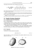
18.14. Elliptic Functions
An elliptic function is a function that is the inverse of an elliptic integral. An elliptic function
is a doubly periodic meromorphic function of a complex variable. All its periods can be
written in the form 2mω
1
+ 2nω
2
with integer m and n,whereω
1
and ω
2
are a pair of
(primitive) half-periods. The ratio τ = ω
2
/ω
1
is a complex quantity that may be considered
to have a positive imaginary part, Im τ > 0.
Throughout the rest of this section, the following brief notation will be used: K = K(k)
and K
= K(k
) are complete elliptic integrals with k
=
√
1 – k
2
.
18.14.1. Jacobi Elliptic Functions
18.14.1-1. Definitions. Simple properties. Special cases.
When the upper limit ϕ of the incomplete elliptic integral of the first kind
u =
ϕ
0
dα
√
1 – k
2
sin
2
α
= F (ϕ, k)
is treated as a function of u, the following notation is used:
u =amϕ.
18.14. ELLIPTIC FUNCTIONS 973
Naming: ϕ is the amplitude and u is the argument.
Jacobi elliptic functions:
sn u =sinϕ =sinamu (sine amplitude),
cn u =cosϕ =cosamu (cosine amplitude),
dn u =
1 – k
2
sin
2
ϕ =
dϕ
du
(delta amlplitude).
Along with the brief notations sn u,cnu,dnu, the respective full notations are also used:
sn(u, k), cn(u, k), dn(u, k).
Simple properties:
sn(–u)=–snu,cn(–u)=cnu,dn(–u)=dnu;
sn
2
u +cn
2
u = 1, k
2
sn
2
u +dn
2
u = 1,dn
2
u – k
2
cn
2
u = 1 – k
2
,
where i
2
=–1.
Jacobi functions for special values of the modulus (k = 0 and k = 1):
sn(u, 0)=sinu,cn(u, 0)=cosu,dn(u, 0)=1;
sn(u, 1)=tanhu,cn(u, 1)=
1
cosh u
,dn(u, 1)=
1
cosh u
.
Jacobi functions for special values of the argument:
sn(
1
2
K, k)=
1
√
1 + k
,cn(
1
2
K, k)=
k
1 + k
,dn(
1
2
K, k)=
√
k
;
sn(K, k)=1,cn(K, k)=0,dn(K, k)=k
.
18.14.1-2. Reduction formulas.
sn(u K)=
cn u
dn u
,cn(u K)= k
sn u
dn u
, dn(u K)=
k
dn u
;
sn(u 2 K)=–snu,cn(u 2 K)=–cnu, dn(u 2 K)=dnu;
sn(u + i K
)=
1
k sn u
,cn(u + i K
)=–
i
k
dn u
sn u
, dn(u + i K
)=–i
cn u
sn u
;
sn(u + 2i K
)=snu,cn(u + 2i K
)=–cnu, dn(u + 2i K
)=–dnu;
sn(u + K +i K
)=
dn u
k cn u
,cn(u + K+i K
)=–i
k
k cn u
, dn(u + K+i K
)=ik
sn u
cn u
;
sn(u + 2 K +2i K
)=–snu,cn(u + 2 K +2i K
)=cnu, dn(u + 2 K +2i K
)=–dnu.
18.14.1-3. Periods, zeros, poses, and residues.
TABLE 18.4
Periods, zeros, poles, and residues of the Jacobian elliptic functions
( m, n = 0,
1, 2, ; i
2
=–1)
Functions Periods Zeros Poles Residues
sn u
4m K +2n K
i 2m K +2n K
i
2m K +(2n +1) K
i
(–1)
m
1
k
cn u
(4m+2n) K+2n K
i (2m+1) K+2n K
i 2m K +(2n +1) K
i
(–1)
m–1
i
k
dn u
2m K +4n K
i
(2m+1) K+(2n+1) K
i 2m K +(2n +1) K
i
(–1)
n–1
i
974 SPECIAL FUNCTIONS AND THEIR PROPERTIES
18.14.1-4. Double-argument formulas.
sn(2u)=
2 sn u cn u dn u
1 – k
2
sn
4
u
=
2 sn u cn u dn u
cn
2
u +sn
2
u dn
2
u
,
cn(2u)=
cn
2
u –sn
2
u dn
2
u
1 – k
2
sn
4
u
=
cn
2
u –sn
2
u dn
2
u
cn
2
u +sn
2
u dn
2
u
,
dn(2u)=
dn
2
u – k
2
sn
2
u cn
2
u
1 – k
2
sn
4
u
=
dn
2
u +cn
2
u (dn
2
u – 1)
dn
2
u –cn
2
u (dn
2
u – 1)
.
18.14.1-5. Half-argument formulas.
sn
2
u
2
=
1
k
2
1 –dnu
1 +cnu
=
1 –cnu
1 +dnu
,
cn
2
u
2
=
cn u +dnu
1 +dnu
=
1 – k
2
k
2
1 –dnu
dn u –cnu
,
dn
2
u
2
=
cn u +dnu
1 +cnu
=(1 – k
2
)
1 –cnu
dn u –cnu
.
18.14.1-6. Argument addition formulas.
sn(u v)=
sn u cn v dn v sn v cn u dn u
1 – k
2
sn
2
u sn
2
v
,
cn(u
v)=
cn u cn v sn u sn v dn u dn v
1 – k
2
sn
2
u sn
2
v
,
dn(u
v)=
dn u dn v k
2
sn u sn v cn u cn v
1 – k
2
sn
2
u sn
2
v
.
18.14.1-7. Conversion formulas.
Table 18.5 presents conversion formulas for Jacobi elliptic functions. If k > 1,then
k
1
= 1/k < 1. Elliptic functions with real modulus can be reduced, using the first set of
conversion formulas, to elliptic functions with a modulus lying between 0 and 1.
18.14.1-8. Descending Landen transformation (Gauss’s transformation).
Notation:
μ =
1 – k
1 + k
, v =
u
1 + μ
.
Descending transformations:
sn(u, k)=
(1 + μ)sn(v, μ
2
)
1 + μ sn
2
(v, μ
2
)
,cn(u, k)=
cn(v, μ
2
)dn(v, μ
2
)
1 + μ sn
2
(v, μ
2
)
,dn(u, k)=
dn
2
(v, μ
2
)+μ – 1
1 + μ –dn
2
(v, μ
2
)
.
18.14. ELLIPTIC FUNCTIONS 975
TABLE 18.5
Conversion formulas for Jacobi elliptic functions. Full notation is used: sn(u, k), cn(u, k), dn(u, k)
u
1
k
1
sn(u
1
, k
1
) cn(u
1
, k
1
) dn(u
1
, k
1
)
ku
1
k
k sn(u, k) dn(u, k) cn(u, k)
iu
k
i
sn(u, k)
cn(u, k)
1
cn(u, k)
dn(u, k)
cn(u, k)
k
u
i
k
k
k
sn(u, k)
dn(u, k)
cn(u, k)
dn(u, k)
1
dn(u, k)
iku
i
k
k
ik
sn(u, k)
dn(u, k)
1
dn(u, k)
cn(u, k)
dn(u, k)
ik
u
1
k
ik
sn(u, k)
cn(u, k)
dn(u, k)
cn(u, k)
1
cn(u, k)
(1 +k)u
2
√
k
1 +k
(1 +k)sn(u, k)
1 +k sn
2
(u, k)
cn(u, k)dn(u, k)
1 +k sn
2
(u, k)
1 –k sn
2
(u, k)
1 +k sn
2
(u, k)
(1 +k
)u
1 –k
1 +k
(1 +k
)sn(u, k)cn(u, k)
dn(u, k)
1 –(1 +k
)sn
2
(u, k)
dn(u, k)
1 –(1 –k
)sn
2
(u, k)
dn(u, k)
18.14.1-9. Ascending Landen transformation.
Notation:
μ =
4k
(1 + k)
2
, σ =
1 – k
1 + k
, v =
u
1 + σ
.
Ascending transformations:
sn(u, k)=(1 +σ)
sn(v, μ)cn(v, μ)
dn(v, μ)
,cn(u, k)=
1 +σ
μ
dn
2
(v, μ)–σ
dn(v, μ)
,dn(u, k)=
1 –σ
μ
dn
2
(v, μ)+σ
dn(v, μ)
.
18.14.1-10. Series representation.
Representation Jacobi functions in the form of power series in u:
sn u = u –
1
3!
(1 + k
2
)u
3
+
1
5!
(1 + 14k
2
+ k
4
)u
5
–
1
7!
(1 + 135k
2
+ 135k
4
+ k
6
)u
7
+ ··· ,
cn u = 1 –
1
2!
u
2
+
1
4!
(1 + 4k
2
)u
4
–
1
6!
(1 + 44k
2
+ 16k
4
)u
6
+ ··· ,
dn u = 1 –
1
2!
k
2
u
2
+
1
4!
k
2
(4 + k
2
)u
4
–
1
6!
k
2
(16 + 44k
2
+ k
4
)u
6
+ ··· ,
am u = u –
1
3!
k
2
u
3
+
1
5!
k
2
(4 + k
2
)u
5
–
1
7!
k
2
(16 + 44k
2
+ k
4
)u
7
+ ··· .
These functions converge for |u| < |K(k
)|.
Representation Jacobi functions in the form of trigonometric series:
sn u =
2π
k K
√
q
∞
n=1
q
n
1 – q
2n–1
sin
(2n – 1)
πu
2 K
,