Handbook of mathematics for engineers and scienteists part 151 doc

1018 CALCULUS OF VARIATIONS AND OPTIMIZATION
The rules for constructing the dual problem are as follows:
1. In all constraints of the primal problem, the constant terms must be on the right-hand
side, and the terms with the unknowns must be on the left-hand side.
2. All inequality constraints must have the same inequality signs.
3. The matrix
A =
⎛
⎜
⎜
⎝
a
11
a
12
··· a
1n
a
21
a
22
··· a
2n
.
.
.
.
.
.
.
.

.
.
.
.
a
m1
a
m2
··· a
mn
⎞
⎟
⎟
⎠
of coefficients of the unknowns in the system of constraints (19.2.1.12) of the primal
problem and the similar matrix
A
T
=
⎛
⎜
⎜
⎝
a
11
a
21
··· a
m1
a

12
a
22
··· a
m2
.
.
.
.
.
.
.
.
.
.
.
.
a
1n
a
2n
··· a
mn
⎞
⎟
⎟
⎠
for the dual problem are obtained from each other by transposition.
4. If the inequality constraints of the primal problem have the ≤ signs, then the objective
function Z(x) must be maximized; if the signs are ≥, then the objective function Z(x)

must be minimized.
5. To each constraint in the primal problem, there corresponds an unknown in the dual
problem. The unknown corresponding to an inequality constraint must be nonnegative,
and the unknown corresponding to an equality constraint may have any sign.
6. The number of variables in the dual problem is equal to the number of functional
constraints (19.2.1.12) in the primal problem, and the number of constraints in sys-
tem (19.2.1.15) of the dual problem is equal to the number of variables in the primal
problem.
7. The coefficients of the unknowns in the objective function (19.2.1.14) of the dual
problem are equal to the constant terms in system (19.2.1.12) of constraints in the
primal problem. The right-hand sides of constraints (19.2.1.15) in the dual problem are
equal to the coefficients of the unknowns in the objective function (19.2.1.11) of the
primal problem.
8. The objective function W (y) of the dual problem is to be minimized if Z(x)istobe
maximized (i.e., if Z(x) → max, then W (y) → min), and vice versa.
Duality theorems establish a relationship between the optimal solutions of a pair of dual
problems.
F
IRST DUALITY THEOREM.
For a pair of mutually dual linear programming problems,
one of the following alternative cases holds:
1.
If one of the problems has an optimal solution, then so does the other, and the objective
values on the optimal solutions are the same for both problems.
2.
If one of the problems is unbounded, then the other is infeasible.
SECOND DUALITY THEOREM.
Let
x =(x
1

, , x
n
)
be a feasible solution of the primal
problem (
19.2.1.11)–(19.2.1.13), and let y =(y
1
, , y
m
) be a feasible solution of the dual
problem (19.2.1.14)–(19.2.1.16). These solutions are optimal in the respective problems if
and only if
x
j

m

i=1
a
ij
y
i
– c
j

= 0 (j = 1, 2, , n); (19.2.1.17)
19.2. MAT H E M AT I CAL PROGRAMMING 1019
y
i


n

j=1
a
ij
x
j
– b
i

= 0 (i = 1, 2, , m). (19.2.1.18)
In other words, if the ith constraint in the primal problem is inactive (holds with strict
inequality) for an optimal solution of the primal problem, then the ith coordinate of the
optimal solution of the dual problem is zero, and, conversely, if the ith coordinate of the
optimal solution of the dual problem is nonzero, then the ith constraint in the primal problem
is active (holds with equality) for the optimal solution of the primal problem.
Example 4. Suppose that the primal problem has the form
Z(x)=–2x
1
+ 4x
2
+ 14x
3
+ 2x
4
→ min,
– 2x
1
– x
2

+ x
3
+ 2x
4
= 6,
– x
1
+ 2x
2
+ 4x
3
– 5x
4
= 30,
x
j
≥ 0 (j = 1, 2, 3, 4).
Then the dual problem is
W (y)=6y
1
+ 30y
2
→ max,
– 2y
1
– y
2
≤ –2,
– y
1

+ 2y
2
≤ 4,
y
1
+ 4y
2
≤ 14,
2y
1
– 5y
2
≤ 2.
The optimal solution of the dual problem is y
opt
=(2, 3). After the substitution of the optimal solution into
the system of constraints in the dual problem, we see that the first and last constraints are satisfied with strict
inequality,
– 2×2– 3 <–2 ⇒ x
∗
1
= 0,
– 2 + 2×3= 4 ⇒ x
∗
2
> 0,
2 + 4×3= 14 ⇒ x
∗
3
> 0,

2×2– 5×3< 2 ⇒ x
∗
4
= 0.
By the second duality theorem, the corresponding coordinates of the optimal solution of the primal problem
are zero, x
∗
1
= x
∗
4
= 0. The system of constraints of the primal problem acquires the form
– x
2
+ x
3
= 6,
2x
2
+ 4x
3
= 30,
which implies that x
∗
2
= 1, x
∗
3
= 7.
Thus x

opt
=(0, 1, 7, 0) is the optimal solution of the primal problem.
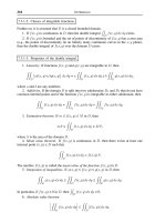
19.2.1-5. Transportation problem. General statement of problem.
Suppose that m supply sources A
1
, , A
m
have amounts a
1
, , a
m
of identical goods
that must be shipped to n consumers B
1
, , B
n
with respective demands b
1
, , b
n
for
these goods. Let c
ij
(i = 1, 2, , m; j = 1, 2, , n) be the unit transportation cost from
supply source i to consumer destination j. The problem is to find a flow of least cost that
ships from supply sources to consumer destinations.
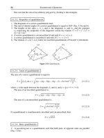
The input data of the transportation problem are usually presented in the form of the
table shown in Fig. 19.1.
Let x
ij

(i = 1, 2, , m; j = 1, , n)betheflow from supply source i to consumer
destination j.Themathematical model of the transportation problem in the general case
has the form
Z(x)=
m

i=1
n

j=1
c
ij
x
ij
→ min, (19.2.1.19)
1020 CALCULUS OF VARIATIONS AND OPTIMIZATION
Figure 19.1. The input data of the transportation problem.
n

j=1
x
ij
= a
i
(i = 1, 2, , m), (19.2.1.20)
m

i=1
x
ij

= b
j
(j = 1, 2, , n), (19.2.1.21)
x
ij
> 0, a
i
≥ 0, b
j
≥ 0 (i = 1, 2, , m; j = 1, 2, , n). (19.2.1.22)
The objective function (19.2.1.19) is the total transportation cost to be minimized. Equa-
tions (19.2.1.20) mean that each supply source must ship all goods present at that source.
Equations (19.2.1.21) mean that the demands of all consumers must be completely satisfied.
Inequalities (19.2.1.22) are the conditions that all variables in the problem are nonnegative.
A necessary and sufficient condition for the solvability of (19.2.1.19)–(19.2.1.22) is the
balance condition
m

i=1
a
i
=
n

j=1
b
j
.(19.2.1.23)
A transportation problem satisfying relation (19.2.1.23) is said to be balanced,andthe
corresponding model is said to be closed. If this relation does not hold, then the problem is

said to be unbalanced and the corresponding model is said to be open.
Under the balance condition (19.2.1.23), the rank of the system of equations (19.2.1.20),
(19.2.1.20) is equal to n + m – 1; therefore, n + m – 1 out of the mn unknown variables
must be basic variables. It follows that for any feasible basic flow the number of occupied
cells in the transportation tableau shown in Fig. 19. 1 is equal to n + m – 1; these cells are
usually said to be basic and the other cells are said to be nonbasic.
There are various methods for obtaining a feasible initial solution (a feasible shipment)
in the transportation problem, including the cross-out method, the northwest corner rule, the
minimal cost method, Vogel’s approximation method, etc. Of these methods, the minimal
cost method is simplest and most convenient.
Minimal cost method. The method consists of several steps of the same type. At each
step, one fills only one cell in the tableau corresponding to the minimal cost min
i,j
{c
ij
} and
excludes only one row (supply source) or column (consumer destination) from subsequent
considerations. A supply source is excluded if its supply of goods is completely exhausted.
A consumer is eliminated if his demand is completely satisfied. At each step, either a supply
source or a consumer is excluded. If a supply source is yet to be excluded but its supply of
19.2. MAT H E M AT I CAL PROGRAMMING 1021
goods is already zero, then, at the step where it should (but cannot) supply goods, a basic
zero is written in the corresponding cell and only after this the supply source is excluded.
Consumers are treated similarly.
Reduction of an unbalanced transportation problem to a balanced transportation prob-
lem.
1. If the total supply exceeds the total demand, i.e.,
m

i=1

a
i
>
n

j=1
b
j
,
then one introduces fictitious consumer n + 1 with demand
b
n+1
=
m

i=1
a
i
–
n

j=1
b
j
equal to the difference between the total supply and total demand and with zero unit
transportation costs c
i(n+1)
= 0 (i = 1, 2, , m).
2. If the total demand exceeds the total supply, i.e.,
m


i=1
a
i
<
n

j=1
b
j
,
then one introduces fictitious supply source m + 1 with supply
a
m+1
=
n

j=1
b
j
–
m

i=1
a
i
equal to the difference between the total demand and the total supply and with zero unit
transportation costs c
(m+1)j
= 0 (j = 1, 2, , n).

Remark. When constructing the initial basic solution, the supply of the fictitious source and the demands
of the fictitious consumer are the last to be assigned, even though they correspond to minimum (zero) unit
transportation costs.
19.2.1-6. Method of potentials.
A balanced transportation problem can be solved as a linear programming problem. But
there are less cumbersome methods for solving the transportation problem. The most widely
used method is the method of potentials.
If a feasible solution X ≡ [x
ij
](i = 1, 2, , m; j = 1, 2, , n) of the transportation
problem is optimal, then there exist supplier potentials u
i
(i = 1, 2, , m) and consumer
potentials v
j
(j = 1, 2, , n) satisfying the following conditions:
u
i
+ v
j
= c
ij
for basic cells, (19.2.1.24)
u
i
+ v
j
≤ c
ij
for nonbasic cells. (19.2.1.25)

Relations (19.2.1.24) are used as a system of equations for the potentials. This system has
n + m unknowns and n + m – 1 equations. Since the number of unknowns exceeds the
number of equations by one, one of the variables can be taken arbitrarily, and the others are
then found from the system.
Inequalities (19.2.1.25) are used to verify the optimality of a basic solution. To this end,
the reduced costs
Δ
ij
= u
i
+ v
j
– c
ij
(19.2.1.26)
of nonbasic cells are used.
1022 CALCULUS OF VARIATIONS AND OPTIMIZATION
Remark 1. For basic cells, the quantities Δ
ij
are zero, Δ
ij
= 0.
Remark 2. The variables u
i
(i = 1, 2, , m) are dual to the respective constraints in (19.2.1.20), and the
variables v
j
(j = 1, 2, , n) are dual to the respective constraints in (19.2.1.21). The dual problem has the
form
m


i=1
a
i
u
i
+
n

j=1
b
j
v
j
→ min,
u
i
+ v
j
≤ c
ij
(i = 1, 2, , m, j = 1, 2, , n).
THEOREM (AN OPTIMALITY CRITERION).
An admissible solution is optimal if the reduced
costs are nonpositive for all cells in the tableau.
A cycle is a sequence (i
1
, j
1
), (i

1
, j
2
), (i
2
, j
2
), ,(i
k
, j
1
) of cells in the transportation
problem tableau in which exactly two neighboring cells lie in the same row or column and,
moreover, the first and last cells also lie in the same row or column.
If the current basic solution is not optimal, then one needs to pass to a new solution with
smaller value of the objective function. To this end, in the tableau one takes the cell with
the largest positive reduced cost
max{Δ
ij
} = Δ
lk
.
Next, one constructs a cycle including this cell and some basic cells. The cells in the cycle
are alternately marked by “+” and “–” signs starting from the cell with the largest positive
reduced cost. For the “–” cells, one finds the quantity θ =min{x
ij
}. Next, one performs a
shift (redistribution of goods) over the cycle by θ. The “–” cell at which min{x
ij
} is attained

becomes empty. If the minimum is attained at several cells, then one of them becomes empty
and the other cells are filled with basic zeros, so that the number of occupied cells remains
equal to n + m – 1.
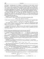
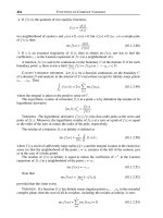
Example 5. Let us solve the transportation problem with the following input data (see Fig. 19.2):
Figure 19.2. Input data for Example 5.
The total demand
4

j=1
b
j
= 200+200+300+400 = 1100 exceeds the total supply
3

i=1
a
i
= 200+300+500 =1000
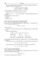
by 100 units; hence the transportation problem is unbalanced. One should introduce the fictitious fourth supply
source with supply a
4
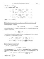
= 100 and with zero unit transportation costs (see Fig. 19.3).
The initial basic solution x
1
is found by the minimal cost method (Fig. 19.3). On this solution, the objective
function takes the value
Z(x
1
)=1 × 200 + 2 × 200 + 3 × 100 + 7 × 100 + 9 × 300 + 12 × 100 + 0 × 100 = 5300.
19.2. MAT H E M AT I CAL PROGRAMMING 1023

Figure 19.3. Introduction of the fictitious fourth supply source. The initial basis solution.
To verify whether the basic solution is optimal, we find the potentials. To this end, we use system (19.2.1.24),
which acquires the form
u
1
+ v
4
= 1,
u
2
+ v
1
= 2,
u
2
+ v
2
= 3,
u
3
+ v
2
= 7,
u
3
+ v
3
= 9,
u
3

+ v
4
= 12,
u
4
+ v
4
= 0.
Let u
3
= 0. Then the other potentials are determined uniquely: v
2
= 7, v
3
= 9, v
4
= 12, u
1
=–11, u
4
=–12,
u
2
=–4,andv
1
= 6. The values of the potentials are written down in the tableau for the solution of the
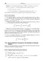
transportation problem (see Fig. 19.4).
Figure 19.4. Determination of potentials. Construction of the cycle.
Next, we verify whether the solution x
1

is optimal. To this end, using (19.2.1.26), we find the reduced
costs Δ
ij
for all empty (nonbasic) cells of the tableau. The solution x
1
is not optimal since there is a positive
reduced cost Δ
24
= u
2
+ v
4
– c
24
=–4 + 12 – 6 = 2.
For cell (2, 4) with positive reduced cost, we construct the cycle (2, 4), (3, 4), (3, 2), (2, 2), (2, 4). The cycle
is shown in Fig. 19.4. At the corners of the cycle, we alternately write the “+” and “–” signs, starting from cell
(2, 4). For the cells with the “–” sign, we have θ =min{100, 100}. Then we perform a shift (redistribution of
1024 CALCULUS OF VARIATIONS AND OPTIMIZATION
Figure 19.5. The second basis solution.
goods) over the cycle by θ = 100 and obtain the second basic solution x
2
(see Fig. 19.5). Once the system of
potentials has been found (Fig. 19.5), we see that the solution x
2
is optimal. The objective function takes the
value
Z(x
2
)=1 × 200 + 2 × 200 + 6 × 100 + 7 × 200 + 9 × 300 + 0 × 100 = 5200

on this solution. Thus, Z
min
(X)=5200 for
X
∗
=

000200
200 0 0 100
0 200 300 0

.
19.2.1-7. Game theory.
Mathematical models of conflict situations are called games, and their participants are
called players. Mathematical models of conflict situations and various methods for solving
problems that arise in these situations are constructed in game theory.
According to the number of players, the games are divided into two-person and n-
person games.Inn-person games, the players’ interests may coincide. In this case, they
can cooperate and form coalitions. Such games are called coalition games.
Aplayer’sstrategy is a set of rules uniquely determining the player’s behavior in each
specific situation arising in the game. A strategy ensuring the maximum possible mean
payoff for a player in repeated games is said to be optimal. The number of possible strategies
of each player can be either finite or infinite. Depending on this, the games are divided into
finite and infinite games.
Games in which one of the players is indifferent to the results are usually called “games
with nature.”
A two-person game in which the payoff of one player is equal to the loss of the other
player is called an antagonistic two-person zero-sum game. Suppose that two players A
and B have finitely many pure strategies: player A can choose any of m strategies A
1

, ,
A
m
, and player B can choose any of n strategies B
1
, , B
n
. These strategies determine
the payoff matrix
⎛
⎜
⎜
⎝
a
11
a
12
··· a
1n
a
21
a
22
··· a
2n
.
.
.
.
.

.
.
.
.
.
.
.
a
m1
a
m2
··· a
mn
⎞
⎟
⎟
⎠
,(19.2.1.27)