Handbook of mathematics for engineers and scienteists part 162 pps

21.3. STATISTIC AL HYPOTHESIS TESTING 1095
Example 1. The hypothesis that the theoretical distribution function is normal with zero expectation is a
parametric hypothesis.
Example 2. The hypothesis that the theoretical distribution function is normal is a nonparametric hypoth-
esis.
Example 3. The hypothesis H
0
that the variance of a random variable X is equal to σ
2
0
, i.e., H
0
:Var{X} =
σ
2
0
, is simple. For an alternative hypothesis one can take one of the following hypotheses: H
1
:Var{X} > σ
2
0
(composite hypothesis), H
1
:Var{X} < σ
2
0
(composite hypothesis), H
1
:Var{X} ≠ σ
2
0

(composite hypothesis),
or H
1
:Var{X} = σ
2
1
(simple hypothesis).
21.3.1-2. Statistical test. Type I and Type II errors.
1
◦
.Astatistical test (or simply a test) is a rule that permits one, on the basis of a sample
X
1
, , X
n
alone, to accept or reject the null hypothesis H
0
(respectively, reject or accept
the alternative hypothesis H
1
). Any test is characterized by two disjoint regions:
1. The critical region W is the region in the n-dimensional space R
n
such that if the
sample X
1
, , X
n
lies in this region, then the null hypothesis H
0

is rejected (and the
alternative hypothesis H
1
is accepted).
2. The acceptance region
W (W = R
n
\W ) is the region in the n-dimensional space R
n
such that if the sample X
1
, , X
n
lies in this region, then the null hypothesis H
0
is
accepted (and the alternative hypothesis H
1
is rejected).
2
◦
. Suppose that there are two hypotheses H
0
and H
1
, i.e., two disjoint subsets Γ
0
and Γ
1
are singled out from the set of all distribution functions. We consider the null hypothesis

H
0
that the sample X
1
, , X
n
is drawn from a population with theoretical distribution
function F (x) belonging to the subset Γ
0
and the alternative hypothesis that the sample is
drawn from a population with theoretical distribution function F (x) belonging to the subset
Γ
1
. Suppose, also, that a test for verifying these hypotheses is given; i.e., the critical region
W and the admissible region W are given. Since the sample is random, there may be errors
of two types:
i) Type I error is the error of accepting the hypothesis H
1
(the hypothesis H
0
is rejected),
while the null hypothesis H
0
is true.
ii) Type II error is the error of accepting the hypothesis H
0
(the hypothesis H
1
is rejected),
while the alternative hypothesis H

1
is true.
The probability α of Type I error is called the false positive rate,orsize of the test, and
is determined by the formula
α = P [(X
1
, , X
n
) W ]
=
⎧
⎨
⎩

P (X
1
)P (X
2
) P(X
n
) in the discrete case,



p(X
1
)p(X
2
) p(X
n

) dx
1
dx
n
in the continuous case;
here P (x)orp(x) is the distribution series or the distribution density of the random vari-
able X under the assumption that the null hypothesis H
0
is true, and the summation or
integration is performed over all points (x
1
, , x
n
) W . The number 1 – α is called the
specificity of the test. If the hypothesis H
0
is composite, then the size α = α[F (x)] depends
on the actual theoretical distribution function F (x) Γ
0
. If, moreover, H
0
is a parametric
hypothesis, i.e., Γ
0
is a parametric family of distribution functions F (x; θ) depending on
the parameter θ with range Θ
0
Θ,whereΘ is the region of all possible values θ, then,
instead of notation α[F (x)], the notation α(θ) is used under the assumption that θ Θ
0

.
1096 MATHE MATIC AL STATISTIC S
The probability

β of Type II error is called the false negative rate.Thepower β = 1 –

β
of the test is the probability that Type II error does not occur, i.e., the probability of rejecting
the false hypothesis H
0
and accepting the hypothesis H
1
. The test power is determined by
the same formula as the test specificity, but in this case, the distribution series P (x)orthe
density function p(x) are taken under the assumption that the alternative hypothesis H
1
is
true. If the hypothesis H
1
is composite, then the power β = β[F(x)] depends on the actual
theoretical distribution function F (x) Γ
1
. If, moreover, H
1
is a parametric hypothesis,
then, instead of the notation β[F (x)], the notation β(θ) is used under the assumption θ Θ
1
,
where Θ
1

is the range of the unknown parameter θ under the assumption that the hypothesis
H
1
is true.
The difference between the test specificity and the test power is that the specificity
1 – α[F (x)] is determined for the theoretical distribution functions F(x)
Γ
0
,andthe
power β(θ) is determined for the theoretical distribution functions F(x)
Γ
1
.
3
◦
. Depending on the form of the alternative hypothesis H
1
, the critical regions are classi-
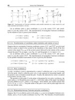
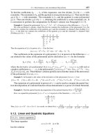
fied as one-sided (right-sided and left-sided) and two-sided:
1. The right-sided critical region (Fig. 21.3a) consisting of the interval (t
R
cr
; ∞), where the
boundary t
R
cr
is determined by the condition
P [S(X
1
, , X

n
)>t
R
cr
]=α;(21.3.1.1)
x
()a ()b ()c
xx
tt tt
cr cr cr cr
RL LR
px() px() px()
Figure 21.3. Right-sided (a), left-sided (b), and two-sided (c) critical region.
2. The left-sided critical region (Fig. 21.3b) consisting of the interval (–∞; t
L
cr
), where the
boundary t
L
cr
is determined by the condition
P [S(X
1
, , X
n
)<t
L
cr
]=α;(21.3.1.2)
3. The two-sided critical region (Fig. 21.3c) consisting of the intervals (–∞; t

L
cr
)and
(t
R
cr
; ∞), where the points t
L
cr
and t
R
cr
are determined by the conditions
P [S(X
1
, , X
n
)<t
L
cr
]=
α
2
and P [S(X
1
, , X
n
)>t
R
cr

]=
α
2
.(21.3.1.3)
21.3.1-3. Simple hypotheses.
Suppose that a sample X
1
, , X
n
is selected from a population with theoretical distribution
function F(x) about which there are two simple hypotheses, the null hypothesis H
0
: F (x)=
F
0
(x) and the alternative hypothesis H
1
: F (x)=F
1
(x), where F
0
(x)andF
1
(x) are known
distribution functions. In this case, there is a test that is most powerful for a given size α;
21.3. STATISTIC AL HYPOTHESIS TESTING 1097
this is called the likelihood ratio test. The likelihood ratio test is based on the statistic called
the likelihood ratio,
Λ = Λ(X
1

, , X
n
)=
L
1
(X
1
, , X
n
)
L
0
(X
1
, , X
n
)
,(21.3.1.4)
where L
0
(X
1
, , X
n
) is the likelihood function under the assumption that the null hypoth-
esis H
0
is true, and L
1
(X

1
, , X
n
) is the likelihood function under the assumption that
the alternative hypothesis H
1
is true.
The critical region W of the likelihood ratio test consists of all points (x
1
, , x
n
)for
which Λ(X
1
, , X
n
) is larger than a critical value C.
N
EYMAN–PEARSON LEMMA.
Of all tests of given size
α
testing two simple hypotheses
H
0
and
H
1
, the likelihood ratio test is most powerful.
21.3.1-4. Sequential analysis. Wald test.
Sequential analysis is the method of statistical analysis in which the sample size is not

fixed in advance but is determined in the course of experiment. The ideas of sequential
analysis are most often used for testing statistical hypotheses. Suppose that observations
X
1
, X
2
, are performed successively; after each trial, one can stop the trials and accept
one of the hypotheses H
0
and H
1
. The hypothesis H
0
is that the random variables X
i
have the probability distribution with density p
0
(x) in the continuous case or the probability
distribution determined by probabilities P
0
(X
i
) in the discrete case. The hypothesis H
1
is that the random variables X
i
have the probability distribution with density p
1
(x)inthe
continuous case or the probability distribution determined by probabilities P

1
(X
i
)inthe
discrete case.
W
ALD TEST.
Of all tests with given size
α
,power
β
, finite mean number
N
0
of
observations under the assumptionthat the hypotheses
H
0
is true, and fi nite mean number
N
1
of observations under the assumption that the hypothesis
H
1
is true, the sequential likelihood
ratio test minimizes both
N
0
and
N

1
.
The decision in the Wald test is made as follows. One specifies critical values A and B,
0 < A < B.TheresultX
1
of the first observation determines the logarithm of the likelihood
ratio
λ(X
1
)=
⎧
⎪
⎨
⎪
⎩
ln
P
1
(X
1
)
P
0
(X
1
)
in the discrete case,
ln
p
1

(X
1
)
p
0
(X
1
)
in the continuous case.
If λ(X
1
) ≥ B, then the hypothesis H
1
is accepted; if λ(X
1
) ≤ A, then the hypothesis H
1
is
accepted; and if A < λ(X
1
)<B, then the second trial is performed. The logarithm of the
likelihood ratio
λ(X
1
, X
2
)=λ(X
1
)+λ(X
2

)
is again determined. If λ(X
1
, X
2
) ≥ B, then the hypothesis H
1
is accepted; if λ(X
1
, X
2
) ≤ A,
then the hypothesisH
1
is accepted; and if A <λ(X
1
, X
2
)<B, then the third trialis performed.
The logarithm of the likelihood ratio
λ(X
1
, X
2
, X
3
)=λ(X
1
)+λ(X
2

)+λ(X
3
)
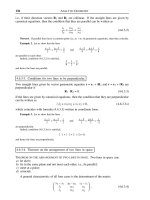
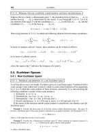
is again determined, and so on. The graphical scheme of trials is shown in Fig. 21.4.
For the size α and the power β of the Wald test, the following approximate estimates
hold:
α ≈
1 – e
A
e
B
– e
A
, β ≈
e
B
(1 – e
A
)
e
B
– e
A
.
1098 MATHE MATIC AL STATISTIC S
A
B
(1, ( ))λX
(2, ( , ))λX X
Acceptance region for hypothesis H

Acceptance region for hypothesis H
1
0
(3,(,,))λXXX
λ
N
1
1
1
1
2
23
2345
Figure 21.4. The graphical scheme of the Wald test.
For given α and β, these estimates result in the following approximate expressions for the
critical values A and B:
A ≈ ln
β
1 – α
, B ≈ ln
β
α
.
For the mean numbers N
0
and N
1
of observations, the following approximate estimates
hold under the assumptions that the hypothesis H
0

or H
1
is true:
N
0
≈
αB +(1 – α)A
M[λ(X)|H
0
]
, N
1
≈
βB +(1 – β)A
M[λ(X)|H
1
]
,
where
E{λ(X)|H
0
} =
L

i=1
ln
P
1
(b
i

)
P
0
(b
i
)
P
0
(b
i
), E{λ(X)|H
1
} =
L

i=1
ln
P
1
(b
i
)
P
0
(b
i
)
P
1
(b

i
)
in the discrete case and
E{λ(X)|H
0
} =

∞
–∞
ln
p
1
(x)
p
0
(x)
p
0
(x) dx, E{λ(X)|H
1
} =

∞
–∞
ln
p
1
(x)
p
0

(x)
p
1
(x) dx
in the continuous case.
21.3.2. Goodness-of-Fit Tests
21.3.2-1. Statement of problem.
Suppose that there is a random sample X
1
, , X
n
drawn from a population X with
unknown theoretical distribution function. It is required to test the simple nonparametric
hypothesis H
0
:F (x)=F
0
(x) against the compositealternative hypothesis H
1
:F (x)≠ F
0
(x),
where F
0
(x) is a given theoretical distribution function. There are several methods for
solving this problem that differ in the form of the measure of discrepancy between the
empirical and hypothetical distribution laws. For example, in the Kolmogorov test (see
Paragraph 21.3.2-2) and the Smirnov test (see Paragraph 21.3.2-3), this measure is a function
of the difference between the empirical distribution function F
∗

(x) and the theoretical
distribution function F (x), i.e.,
ρ = ρ[F
∗
(x)–F (x)];
and in the χ
2
-test, this measure is a function of the difference between the theoretical
probabilities p
T
i
= P (H
i
) of the random events H
1
, , H
L
and their relative frequencies
p
∗
i
= n
i
/n, i.e.,
ρ = ρ(p
T
i
– p
∗
i

).
21.3. STATISTIC AL HYPOTHESIS TESTING 1099
21.3.2-2. Kolmogorov test.
To test a hypothesis concerning the distribution law, the statistic
ρ = ρ(X
1
, , X
n
)=
√
n sup
–∞<x<∞
|F
∗
(x)–F (x)| (21.3.2.1)
is used to measure the compatibility (goodness of fit) of the hypothesis in the Kolmogorov
test. A right-sided region is chosen to be the critical region in the Kolmogorov test. For
a given size α, the boundary t
R
cr
of the right-sided critical region can be found from the
relation
t
R
cr
= F
–1
(1 – α).
Table 21.1 presents values depending on the size and calculated by formula (21.3.2.1).
TABLE 21.1

Boundary of right-sided critical region
α 0.5 0.1 0.05 0.01 0.001
t
R
cr
0.828 1.224 1.385 1.627 1.950
As n →∞, the distribution of the statistic ρ converges to the Kolmogorov distribution
and the boundary t
R
cr
of the right-sided critical region coincides with the (1 – α)-quantile
k
1–α
of the Kolmogorov distribution.
The advantages of the Kolmogorov test are its simplicity and the absence of complicated
calculations. But this test has several essential drawbacks:
1. The use of the test requires considerable a priori information about the theoretical law
of distribution; i.e., in addition to the form of the distribution law, one must know the
values of all parameters of the distribution.
2. The test deals only with the maximal deviation of the empirical distribution function
from the theoretical one and does not take into account the variations of this deviation
on the entire range of the random sample.
21.3.2-3. Smirnov test (ω
2
-test).
In contrast to the Kolmogorov test, the Smirnov test takes the mean value of a function
of the difference between the empirical and theoretical distribution functions on the entire
domain of the distribution function to be the measure of discrepancy between the empirical
distribution functionand the theoretical one; this eliminates thedrawback of the Kolmogorov
test.

In the general case, the statistic
ω
2
= ω
2
(X
1
, , X
n
)=

∞
–∞
[F
∗
(x)–F (x)]
2
dF (x)(21.3.2.2)
is used. Using the series X
∗
1
, , X
∗
n
of order statistics, one can rewrite the statistic ω
2
in
the form
ω
2

=
1
n
n

i=1

F
∗
(X
∗
i
)–
2i – 1
2n

2
+
1
12n
2
.(21.3.2.3)
1100 MATHE MATIC AL STATISTIC S
A right-sided region is chosen to be the critical region in the Smirnov test. For a given
size α, the boundary t
R
cr
of the right-sided critical region can be found from the relation
t
R

cr
= F
–1
(1 – α). (21.3.2.4)
Table 21.2 presents the values of t
R
cr
depending on the size and calculated by formula
(21.3.2.4).
TABLE 21.2
Boundary of right-sided critical region
α 0.5 0.1 0.05 0.01 0.001
t
R
cr
0.118 0.347 0.461 0.620 0.744
As n →∞, the distribution of the statistic ω
2
converges to the ω
2
-distribution and
the boundary t
R
cr
of the right-sided critical region coincides with the (1 – α)-quantile of an
ω
2
-distribution.
21.3.2-4. Pearson test (χ
2

-test).
1
◦
.Theχ
2
-test is used to measure the compatibility (goodness of fit) of the theoretical
probabilities p
k
= P (H
k
) of random events H
1
, , H
L
with their relative frequencies
p
∗
k
= n
k
/n in a sample of n independent observations. The χ
2
-test permits comparing the
theoretical distribution of the population with its empirical distribution.
The goodness of fit is measured by the statistic
χ
2
=
L


k=1
(n
k
– np
k
)
2
np
k
=
L

k=1
n
2
k
np
k
– n,(21.3.2.5)
whose distribution as n →∞tends to the chi-square distribution with v = L – 1 degrees of
freedom. According to the χ
2
-test, there are no grounds to reject the theoretical probabilities
for a given confidence level γ if the inequality χ
2
< χ
2
γ
(v) holds, where χ
2

γ
(v)istheγ-
quantile of a χ
2
-distribution with v degrees of freedom. For v > 30, instead of the chi-
square distribution, one can use the normal distribution of the random variable

2χ
2
with
expectation
√
2v – 1 and variance 1.
Remark. The condition n
k
> 5 is a necessary condition for the χ
2
-test to be used.
2
◦
. χ
2
-test with estimated parameters.
Suppose that X
1
, , X
n
is a sample drawn from a population X with unknown
distribution function F (x). We test the null hypothesis H
0

stating that the population is
distributed according to the law with the distribution function F (x) equal to the function
F
0
(x), i.e., the null hypothesis H
0
: F (x)=F
0
(x) is tested. Then the alternative hypothesis
is H
1
: F(x) ≠ F
0
(x).
In this case, the statistic (21.3.2.5) as n →∞tends to the chi-square distribution with
v = L – q – 1 degrees of freedom, where q is the number of estimated parameters. Thus, for
example, q = 2 for the normal distribution and q = 1 for the Poisson distribution. The null
hypothesis H
0
for a given confidence level α is accepted if χ
2
< χ
2
α
(L – q – 1).
21.3. STATISTIC AL HYPOTHESIS TESTING 1101
21.3.3. Problems Related to Normal Samples
21.3.3-1. Testing hypotheses about numerical values of parameters of normal
distribution.
Suppose that a random sample X

1
, , X
n
is drawn from a population X with normal
distribution. Table 21.3 presents several tests for hypotheses about numerical values of the
parameters of the normal distribution.
TABLE 21.3
Several tests related to normal populations with parameters (a, σ
2
)
No.
Hypothesis
to be tested
Test statistic Statistic distribution
Critical region
for a given size
1
H
0
: a = a
0
,
H
1
: a ≠ a
0
U =
m
∗
– a

σ
√
n
standard normal
|U| > u
1–α/2
2
H
0
: a ≤ a
0
,
H
1
: a > a
0
U =
m
∗
– a
σ
√
n
standard normal
U > u
1–α
3
H
0
: a ≥ a

0
,
H
1
: a < a
0
U =
m
∗
– a
σ
√
n
standard normal
U >–u
1–α
4
H
0
: a = a
0
,
H
1
: a ≠ a
0
T =

n
s

2∗
(m
∗
– a)
t-distribution with
n – 1 degrees of freedom
|T | > t
1–α/2
5
H
0
: a ≤ a
0
,
H
1
: a > a
0
T =

n
s
2∗
(m
∗
– a)
t-distribution with
n – 1 degrees of freedom
T > t
1–α

6
H
0
: a ≥ a
0
,
H
1
: a < a
0
T =

n
s
2∗
(m
∗
– a)
t-distribution with
n – 1 degrees of freedom
T >–t
1–α
7
H
0
: σ
2
= σ
2
0

,
H
1
: σ
2
≠ σ
2
0
χ
2
=
s
2∗
σ
2
0
(n – 1)
χ
2
-distribution with
n – 1 degrees of freedom
χ
2
α/2
> χ
2
1–α/2
,
χ
2

> χ
2
1–α/2
8
H
0
: σ
2
≤ σ
2
0
,
H
1
: σ
2
> σ
2
0
χ
2
=
s
2∗
σ
2
0
(n – 1)
χ
2

-distribution with
n – 1 degrees of freedom
χ
2
> χ
2
1–α
9
H
0
: σ
2
≥ σ
2
0
,
H
1
: σ
2
< σ
2
0
χ
2
=
s
2∗
σ
2

0
(n – 1)
χ
2
-distribution with
n – 1 degrees of freedom
χ
2
< χ
2
α
Remark 1. In items 1–6 σ
2
is known.
Remark 2. In items 1–3 u
α
is α-quantile of standard normal distribution.
21.3.3-2. Goodness-of-fittests.
Suppose that a sample X
1
, , X
n
is drawn from a population X with theoretical distribu-
tion function F (x). It is required to test the composite null hypothesis, H
0
: F (x) is normal
with unknown parameters (a, σ
2
), against the composite alternative hypothesis, H
1

: F (x)
is not normal. Since the parameters a and σ
2
are decisive for the normal law, the sample
mean m
∗
(or X) and the adjusted sample variance s
2∗
are used to estimate these parameters.
1
◦
. Romanovskii test. To test the null hypothesis, the following statistic (Romanovskii
ratio) is used:
ρ
rom
= ρ
rom
(X
1
, , X
n
)=
χ
2
(m)–m
√
2m
,(21.3.3.1)