Hardware and Computer Organization- P2 docx
Bạn đang xem bản rút gọn của tài liệu. Xem và tải ngay bản đầy đủ của tài liệu tại đây (970.32 KB, 30 trang )
Chapter 1
12
ever, according to Mann, a conversion factor of about 38 allows for a rough comparison. Thus,
according to the published results
7
, a 1.0 GHz AMD Athlon processor achieved a SPECint95
benchmark result of 42.9, which roughly compares to a SPECint92 result of 1630. The Digital
Equipment Corporation (DEC) AlphaStation 5/300 is one workstation that has published results
for both benchmark tests. It measures about 280 in the graph of Figure 1.6 and 7.33 according to
the SPECint95 benchmark. Multiplying by 38, we get 278.5, which is in reasonable agreement
with the earlier result. We’ll return to the issue of performance measurements in a later chapter.
Number Systems
How do you represent a number in computer? How do you send that number, whatever it may
be, a char, an int, a float or perhaps a double between the processor and memory, or within
the microprocessor itself? This is a fair question to ask and the answer leads us naturally to
an understanding of why modern digital computers are based on the binary (base 2) number
system. In order to investigate this, consider Figure 1.7.
In Figure 1.7 we’ll do a simple-minded experiment.
Let’s pretend that we can place an electrical voltage
on the wire that represents the number we would
like to transmit between two functional elements of
the computer. The method might work for simple
numbers, but I wouldn’t want to touch the wire if I
was sending 2000.456! In fact, this method would
be extremely slow, expensive and would only work
for a narrow range of values.
However, that doesn’t imply that this method isn’t
used at all. In fact, one of the first families of elec
-
tronic computers was the analog computer. The
analog computer is based upon linear amplifiers,
or the kind of electronic circuitry that you might
find in your stereo receiver at home. The key point
is that variables (in this case the voltages on wires)
can assume an infinite range of values between some limits imposed by the nature of the circuitry.
In many of the early analog computers this range might be between –25 volts and +25 volts. Thus,
any quantity that could be represented as a steady, or time varying voltage within this range could
be used as a variable within an analog computer.
The analog computer takes advantage of the fact that there are electronic circuits that can do the
following mathematical operations:
• Add / subtract
• Log / anti-log
• Multiply / divide
• Differentiate / integrate
Figure 1.7: Representing the value of a
number by the voltage on a wire.
24.56345 V
24.56345
RADIO
SHACK
Direction of signal
Zero volts
(ground)
Introduction and Overview of Hardware Architecture
13
By combining this circuits one after another with intermediate amplification and scaling, real-time
systems could be easily modeled and the solution to complex linear differential equations could be
obtained as the system was operating.
However, the analog computer suffers from the same
limitations as does your stereo system. That is, its
amplification accuracy is not infinitely perfect, so the best
accuracy that could be hoped for is about 0.01%, or about
1 part in 10,000. Figure 1.8 shows an analog computer
of the type used by the United States submarines during
World War II. The Torpedo Data Computer, or TDC,
would take as its inputs the compass heading and speed of
the target ship, the heading and speed of the submarine,
the desired firing distance. The correct speed and heading
was then sent to the torpedoes and they would track the
course, speed and depth transmitted to them by the TDC.
Thus, within the limitations imposed by the electronic
circuitry of the 1940’s, an entire family of computers
based upon the idea of inputs and outputs based upon
continuous variables. In that sense, your stereo amplifier
is an analog computer. An amplifier amplifies
, or boosts an
electrical signal. An amplifier with a
gain of 10, has
an output voltage that is, at every instant of time, 10
times greater than the input voltage. Thus, V
out
= 10
V
in
. Here we have an analog computing block that
happens to be a multiplication block with a constant
multiplier.
Anyway, let’s get back to discussing to number sys
-
tems. We might be able to improve on this method
by breaking the number into more manageable parts
and send a more limited signal range over several
wires at the same time (in parallel). Thus, each wire
would only need to transmit a narrow range of val
-
ues. Figure 1.9 shows how this might work.
In this case, each wire in the bundle represents
a decimal decade and each number that we send
would be represented by the corresponding voltages
on the wires. Thus, instead of needing to transmit
potentially lethal voltages, such as 12,567 volts,
the voltage in each wire would never become greater than that of a 9-volt battery. Let’s stop for a
moment because this approach looks promising. How accurate would the voltage on the wire have
to be in so that the circuitry interprets the number as 4, and not 3 or 5? In Figure 1.7, our voltme-
Figure 1.8: An analog computer from a
WWII submarine. Photo courtesy of www.
fleetsubmarine.com.
Figure 1.9: Using a parallel bundle of wires to
transmit a numeric value in a computer. The
wire’s position in the bundle determines its
digital weight. Each wire carries between 0
volts and 9 volts.
2
4
5
6
3
4
5
4.2
RADIO
SHAC
K
Zero volts
(gro
und)
Chapter 1
14
ter shows that the second wire from the bottom measures 4.2 V, not 4 volts. Is that good enough?
Should it really be 4.000 ± .0005 volts? In all probability, this system might work just fine if each
voltage increment has a “slop” of about 0.3 volts. So we would only need to send 4 volts ± 0.3
volts (3.7–4.3 volts) in order to guarantee that the circuitry received the correct number. What if
the circuit erred and sent 4.5 volts instead? This is too large to be a 4 but too small to be a 5. The
answer is that we don’t know what will happen. The value represented by 4.5 volts is undefined.
Hopefully, our computer works properly and this is not a problem.
The method proposed in Figure 1.9 is actually very close to reality, but it isn’t quite what we need. With
the speed of modern computers, it is still far too difficult to design circuitry that is both fast enough and
accurate enough to switch the voltage on a wire between 10 different values. However, this idea is being
looked at for the next generation of computer memory cells. More on that later, stay tuned!
Modern transistors are excellent switches. They can switch a voltage or a current on or off in tril
-
lionths of a second (picoseconds). Can we make use of this fact? Let’s see. Suppose we extend the
concept of a bundle of wires but let’s restrict even further the values that can exist on any indi
-
vidual wire. Since each wire is controlled by a switch, we’ll switch between nothing (0 volts) and
something (~3 volts). This implies that just two numbers may be carried on each wire, 0 or some
-
thing (not 0). Will it work? Let’s look at Figure 1.10.
Figure 1.10: Sending numbers as binary values. Each arrow represents a wire with the
arrowhead representing the direction of signal transmission. The position of each wire in the
bundle represents its numerical weight. Each row represents an increasing power of 2.
2
0
2
1
2
2
2
3
2
4
2
5
2
6
2
7
2
8
2
9
2
10
2
11
2
12
2
13
2
14
2
15
on 1
off 0
on
1
off 0
off 0
on
1
on 1
on
1
off 0
off 0
off 0
on
1
on
1
on 1
on
1
off 0
In this scenario, the amount of information that we can carry on a single wire is limited to nothing,
0, or something (let’s call something “1” or “on”), so we’ll need a lot of wires in order to transmit
anything of significance. Figure 1.10 shows 16 wires, and
as you’ll soon see, this limits us to numbers between 0
and 65,535 if we are dealing with unsigned numbers, or
the signed range of –32,768 to +32,767. Here the decimal
number 0 would be represented by the binary number
00000000000000 and the decimal number 65,535 would
be represented by the binary number 1111111111111111.
Note: For many years, most standard digital
circuits used 5 volts for a 1. However, as
the integrated circuits became smaller and
denser, the logical voltage levels also had
to be reduced. Today, the core of a modern
Pentium or Athlon processor runs at a
voltage of around 1.7–1.8 volts, not very
different from a standard AA battery.
Introduction and Overview of Hardware Architecture
15
Now we’re finally there. We’ll take advantage of the fact that electronic switching elements, or
transistors, can rapidly switch the voltage on a wire between two values. The most common form
of this is between almost 0 volts and something (about 3 volts). If our system is working properly,
then what we define as “nothing”, or 0, might never exceed about ½ of a volt. So, we can define
the number 0 to be any voltage less than ½ volt (actually, it is usually 0.4 volts). Similarly, if the
number that we define as a 1, would never be less than 2.5 volts, then we have all the information
we need to define our number system. Here, the number 0 is never greater than 0.4 volts and the
number 1 is never less than 2.5 volts. Anything between these two ranges is considered to be unde
-
fined and is not allowed.
It should be mentioned that we’ve been refer
-
ring to “the voltage on a wire.” Just where are
the wires in our computer? Strictly speaking,
we should call the wires “electrical conductors.”
They can be real wires, such as the wires in the
cable that you connect from your printer to the
parallel port on the back of your computer. They
can also be thin conducting paths on printed cir
-
cuit boards within your computer. Finally, they
can be tiny aluminum conductors on the proces
-
sor chip itself. Figure 1.11 shows a portion of a
printed circuit board from a computer designed
by the author.
Notice that some of the integrated circuit’s
(ICs) pins appear have wires connecting them to
another device while others seem to be uncon
-
nected. The reason for this is that this printed circuit board is actually a sandwich made up of five
thinner layers with wires printed on either side, giving a total of ten layers. The eight inner layers
also have a thin insulating layer between then to prevent electric short circuits. During the manu
-
facturing process, the five conducting layers and the four insulating layers are carefully aligned and
bonded together. The resultant, ten-layer printed circuit board is approximately 2.5 mm thick.
Without this multilayer manufacturing technique, it would be impossible to build complex com
-
puter systems because it would not be possible to connect the wires between components without
having to cross a separate wire with a different purpose.
[NOTE: A color version of the following figure is included on the DVD-ROM.] Figure 1.12 shows
us just what’s going on with the inner layers. Here is an X-ray view of another computer system
hardware circuit. This is about the same level of complexity that you might find on the mother-
board of your PC. The view is looking through the layers of the board and the conductive traces on
each layer are shown in a different color.
While this may appear quite imposing, most of the layout was done using computer-aided design
(CAD) software. It would take altogether too much time for even a skilled designer to complete
the layout of this board. Figure 1.13 is a magnification of a smaller portion of Figure 1.12. Here
Figure 1.11: Printed wires on a computer circuit board.
Each wire is actual a copper trace approximately 0.08
mm wide. Traces can be as close as 0.08 mm apart
from each other. The large spots are the soldered
pins of the integrated circuits coming through from
the other side of the board.
Chapter 1
16
you can clearly see the various traces on the dif-
ferent layers. Each printed wire is approximately
0.03 mm wide.
[NOTE: A color version of the following figure is
included on the DVD-ROM.]
If you look carefully
at Figure 1.13, you’ll notice that certain colored
wires touch a black dot and then seem to go off in
another direction as a wire of a different color. The
black dots are called vias, and they represent places
in the circuit where a wire leaves its layer and tra-
verses to another layer. Vias are vertical conductors
that allow signals to cross between layers. Without
vias, wires couldn’t cross each other on the board
without short circuiting to each other. Thus, when
you see a green wire (for purposes of the grayscale
image on this page, the green wire appears as a dot-
ted line) crossing a red wire, the two wires are not
in physical contact with other, but are passing over
each other on different layers of the board. This is
an important concept to keep in mind because we’ll
soon be looking at, and drawing our own electronic
circuit diagrams, called schematic diagrams, and
we’ll need to keep in mind how to represent wires
that appear to cross each other without being physi
-
cally connected, and those wires that are connected
to each other.
Let’s review what we’ve just discussed. Modern digi
-
tal computers use the binary (base 2) number system.
They do so because a number system that has only
two digits in its natural sequence of numbers lends
itself to a hardware system which utilizes switches
to indicate if a circuit is in a “1” state (on) or a “0”
state (off). Also, the fundamental circuit elements
that are used to create complex digital networks
are also based on these principles as logical expres
-
sions. Thus, just as we might say, logically, that an
expression is TRUE or FALSE, we can just as easily
describe it as a “1” (TRUE) or “0” (FALSE). As
you’ll soon see, the association of 1 with TRUE and
0 with FALSE is completely arbitrary, and we may reverse the designations with little or no ill effects.
However, for now, let’s adopt the convention that a binary 1 represents a TRUE or ON condition, and a
binary 0 represents a FALSE or OFF condition. We can summarize this in the following table:
Figure 1.12: An X-ray view of a portion of a
computer systems board.
Figure 1.13: A magnified view of a portion of the
board shown in Figure 1.12.
Introduction and Overview of Hardware Architecture
17
Binary Value Electrical Circuit Value Logical Value
0 OFF FALSE
1 ON TRUE
A Simple Binary Example
Since you have probably never been exposed to electrical circuit diagrams, let’s dive right in.
Figure 1.14 is a simple schematic diagram of a circuit containing a battery, two switches, labeled
A and B, and a light bulb, C. The positive terminal on the battery is labeled with the plus (
+) sign
and the negative battery terminal is labeled with the minus (
–) sign. Think of a typical AA battery
that you might use in your portable MP3 player. The little bump on the end is the positive terminal
and the flat portion on the opposite end is the negative terminal. Referring to Figure 1.11, it might
seem curious that the positive terminal is drawn as a wide line, and the negative terminal is drawn
as a narrow line. There’s a reason for it, but we won’t discuss that here. Electrical Engineering
students are taught the reason for this during their initiation ceremony, but I’m sworn to secrecy.
Figure 1.14: A simple circuit using two switches in series to represent the AND function.
+
-
A
B
C
C = A and B
Battery Sy
mbol
Lightbulb (load)
The light bulb, C, will illuminate when enough current flows through it to heat the filament. We
assume that in electrical circuits such as this one, that current flows from positive to negative.
Thus, current exits the battery at the + terminal and flows through the closed switches (A and B),
then through the lamp, and finally to the – terminal of the battery. Now, you might wonder about
this because, as we all know from our high school science classes, that electrical current is actu
-
ally made up of electrons and electrons, being negatively charged, actually flow from the negative
terminal of the battery to the positive terminal; the reverse direction.
The answer to this apparent paradox is historical precedent. As long as we think of the current as
being positively charged, then everything works out just fine.
Anyway, in order for current to flow through the filament, two things must happen: switch A must
be closed (ON) and switch B must be closed (ON). When this condition is met, the output vari-
able, C, will be ON (illuminated). Thus, we can talk about our first example of a
logical equation:
C = A AND B
This is a very interesting result. We’ve seen two apparently very different consequences of using
switches to build computer systems. The first is that we are lead to having to deal with numbers
as binary (base 2) values and the second is that these switches also allow us to create logical
equations. For now, let’s keep item two as an interesting consequence. We’ll deal with it more
thoroughly in the next chapter. Before we leave Figure 1.14, we should point out that the switches,
A and B, are actuated mechanically. Someone flips the switch to turn it on or off. In general, a
Chapter 1
18
switch is a three-terminal device. There is a control input that determines the signal propagation
between the other two terminals.
Bases
Let’s return to our discussion of the binary number system. We are accustomed to using the deci
-
mal (base 10) number system because we had ten fingers before we had an iMAC®. The base (or
radix
) of a number system is just the number of distinct digits in that number system. Consider the
following table:
Base 2 0,1 Binary
Base 8 0,1,2,3,4,5,6,7 Octal
Base 10 0,1,2,3,4,5,6,7,8,9 Decimal
Base 16 0,1,2,3,4,5,6,7,8,9,A,B,C,D,E,F Hexadecimal
Look at the hexadecimal numbers in the table above. There are 16, distinct digits, 0 through 9 and
A through F, representing the decimal numbers 0 through 15, but expressing them in the hexadeci
-
mal system.
Now, if you’ve ever had your PC lockup with the “blue screen of death,” you might recall seeing
some funny looking letters and numbers on the screen. That cryptic message was trying to show
you an address value in hexadecimal where something bad has just happened. It may be of little
solace to you that from now on the message on the blue screen will not only tell you that a bad
thing has happened and you’ve just lost four hours of work, but with your new-found insight, you
will know where in your PC’s memory the illegal event took place.
When we write a number in binary, octal decimal or hexadecimal, we are representing the num
-
ber in exactly the same way, although the number will look quite different to us, depending upon
the base we’re using. Let’s consider the decimal number 65,536. This happens to be 2
16
. Later,
we’ll see that this has special significance, but for now, it’s just a number. Figure 1.15, shows how
each digit of the number, 65,536, represents the column value multiplied by the numerical weight
of the column. The leftmost, or most significant digit,
is the number 6. The rightmost, or least
significant digit, also happens to be 6. The column weight of the most significant digit is 10,000
(10
4
) so the value in that column is 6 x 10,000, or 60,000. If we multiply out each column value
Figure 1.15: Representing a number in base 10. Going from right to left, each digit multiplies
the value of the base, raised to a power. The number is just the sum of these multiples.
10
4
10
3
10
2
10
1
10
0
6 5 5 3 6
6 x 10
0
= 6
3 x 10
1
= 30
5 x 10
2
= 500
5 x 10
3
= 5000
6 x 10
4
= 60000
+
= 65536
• Notice how each column is weighted by
the value of the base raised to the power
• Notice how each column is weighted by
the value of the base raised to the power
Introduction and Overview of Hardware Architecture
19
and then arrange them as a list of numbers to be added together, as we’ve done on the right side of
Figure 1.15, we can add them together and get the same number as we started with. OK, perhaps
we’re overstating the obvious here, but stay tuned, because it does get better. This little example
should be obvious to you because you’re accustomed to manipulating decimal numbers. The key
point is that the column value happens to be the base value raised to a power that starts at 0 in the
rightmost column and increases by 1 as we move to the left. Since decimal is base 10, the column
weights moving leftward are 1, 10, 100, 1000, 10000 and so on.
If we can generalize this method of representing number, then it follows that we would use the
same method to represent numbers in any other base.
Translating Numbers Between Bases
Let’s repeat the above exercise, but this time we’ll use a binary number. Let’s consider the 8-bit
binary number 10101100. Because this number has 8 binary numbers, or bits associated with it,
we call it an 8-bit number. It is customary to call an 8-bit binary number a
byte (in C or C++ this
is a char). It should now be obvious to you why binary numbers are all 1’s and 0’s. Aside from the
fact that these happen to be the two states of our switching circuits (transistors) they are the only
numbers available in a base 2 number system.
The byte is perhaps most notable because we measure storage capacity in byte-size chunks (sorry).
The memory in your PC is probably at least 256 Mbytes (256 million bytes) and your hard disk
has a capacity of 40 Gbytes (40 billion bytes), or more.
Consider Figure 1.16. We use the same method as we used in the decimal example of Figure 1.15.
However, this time the column weight is a multiple of base 2, not base 10. The column weights
go from 2
7
, or 128, the most significant digit, down to 2
0
, or 1. Each column is smaller by a power
of 2. To see what this binary number is in decimal, we use the same process as we did before; we
multiply the number in the column by the weight of the column.
Figure 1.16: Representing a binary number in terms of the powers of the base 2. Notice that
the bases of the octal (8) and hexadecimal (16) number systems are also powers of 2.
2
7
2
6
2
5
2
4
2
3
2
2
2
1
2
0
128 64 32 16 8 4 2 1
Ba
ses of Hex and Octal
1 0 1 0 1 1 0 0
1 x 2
7
= 128
0 x
2
6
= 0
1 x
2
5
= 32
0 x
2
4
= 0
1 x
2
3
= 8
1 x
2
2
= 4
0 x
2
1
= 0
0 x
2
0
= 0
10101100 = 172
172
2 10
Chapter 1
20
Thus, we can conclude that the decimal number 172 is equal to the binary number 10101100. It is
also noteworthy that the bases of the hexadecimal (Hex) number system, 16 and the octal number
system, 8, are also 2
4
and 2
3
, respectively. This might give you a hint as to why we commonly use
the hexadecimal representation and the less common octal representation instead of binary when
we are dealing with our computer system. Quite simply, writing binary numbers gets extremely
tedious very quickly and is highly prone to human errors.
To see this in all of its stark reality, consider the binary equivalent of the decimal value:
2,098,236,812
In binary, this number would be written as:
1111101000100001000110110001100
Now, binary numbers are particularly easy to convert to decimal by this process because the
number is either 1 or 0. This makes the multiplication easy for those of us who can’t remember the
times tables because our PDA’s have allowed significant portions of our cerebral cortex to atrophy.
Since there seems to be a connection between the bases 2, 8 and 16, then it is reasonable to assume
that converting numbers between the three bases would be easier than converting to decimal, since
base 10 is not a natural power of base 2. To see how we convert from binary to octal consider
Figure 1.17.
Figure 1.17: Translating a binary number into an octal number. By factoring
out the value of the base, we can combine the binary number into groups of
three and write down the octal number by inspection.
128 64 32 16 8 4 2 1
1 0 1 0 1 1 0 0
0 thru 7
0 thru 56
0 thru 192
8
2
8
1
8
0
4 x 8
0
= 4
5 x
8
1
= 40
2 x
8
2
= 128
172
2
7
2
6
2
5
2
4
2
3
2
2
2
1
2
0
2
6
(2
1
2
0
)
2
3
( 2
2
2
1
2
0
) 2
0
( 2
2
2
1
2
0
)
Figure 1.17 takes the example of Figure 1.16 one step further. Figure 1.17 starts with the same
binary number, 10101100, or 172 in base 10. However, simple arithmetic shows us that we can
factor out various powers of 2 that happen to also be powers of 8. Consider the dark gray high
-
lighted stripe in Figure 1.17. We can make the following simplifications.
Since any number to the 0 power = 1,
(2
2
2
1
2
0
) = 2
0
× (2
2
2
1
2
0
)
Introduction and Overview of Hardware Architecture
21
Thus,
2
0
= 8
0
= 1
We can perform the same simplification with the next group of three binary numbers:
(2
5
2
4
2
3
) = 2
3
× (2
2
2
1
2
0
)
since 2
3
is a common factor of the group.
However, 2
3
= 8
1
, which is the column weight of the next column in the octal number system.
If we repeat this exercise one more time with the final group of two numbers, we see that:
(2
7
2
6
) = 2
6
× (2
1
2
0
)
since 2
6
is a common factor of the group. Again, 2
6
= 8
2
, which is just the column weight of the
next column in the octal number system.
Since there is this natural relationship between base 8 and base 2, it is very easy to translate numbers
between the bases. Each group of three binary numbers, starting from the right side (least significant
digit) can be translated to an octal digit from 0 to 7 by simply looking at the binary value and writing
down the equivalent octal value. In Figure 1.14, the rightmost group of three binary numbers is 100.
Referring to the column weights this is just 1 * (1 * 4 + 0 * 2 + 0 * 1), or 4. The middle group of
three gives us 8 * (1 * 4 + 0 * 2 + 1 * 1), or 8 * 5 (40). The two remaining numbers gives us 64 *
(1 * 2 + 0 * 1) or 128. Thus, 4 + 40 + 128 = 172, our binary number from Figure 1.8. But where’s
the octal number? Simple, each group of three binary numbers gave us the column value of the
octal digit, so our binary number is 254. Therefore, 10101100 in binary is equal to 254 in octal,
which equals 172 in decimal.
Neat! Thus, we can convert between binary and octal as follows:
• If the number is in octal, write each octal digit in terms of three binary digits. For example:
256773 = 10 101 110 111 111 011
• If the number is in binary, then gather the binary digits into groups of three, starting from
the least significant digit and write down the octal (0 through 7) equivalent. For example:
110001010100110111
2
= 110 001 010 100 110 111 = 612467
8
• If the most significant grouping of binary digits has only 1 or 2 digits remaining, just pad
the group with 0’s to complete a group of three for the most significant octal digit.
Today, octal is not as commonly used as it once was, but you will still see it used occasionally. For
example, in the UNIX (Linux) command
chmod 777, the number 777 is the octal representa-
tion of the individual bits that define file status. The command changes the file permissions for the
users who may then have access to the file.
We can now extend our discussion of the relationship between binary numbers and octal numbers
to consider the relationship between binary and hexadecimal. Hexadecimal (hex) numbers are con
-
verted to and from binary in exactly the same way as we did with octal numbers, except that now
we use 2
4
, as the common factor rather than 2
3
. Referring to Figure 1.18, we see the same process
for hex numbers as we used for octal.
Chapter 1
22
In this case, we factor out the common power of the base, 2
4
, and we’re left with a repeating group
of binary numbers with column values represented as
2
3
2
2
2
1
2
0
It is simple to see that the binary number 1111 = 15
10
, so groups of four binary digits may be
used to represent a number between 0 and 15 in decimal, or 0 through F in hex. Referring back to
Figure 1.16, now that we know how to do the conversion, what’s the hex equivalent of 10101100?
Referring to the leftmost group of 4 binary digits, 1010, this is just 8 + 0 + 2 + 0, or A. The right
-
most group, 1100 equals 8 + 4 + 0 + 0, or C. Therefore, our number in hex is AC.
Let’s do a 16-bit binary number conversion example.
Binary number: 0101111111010111
Octal: 0 101 111 111 010 111 = 057727 (grouped by threes)
Hex: 0101 1111 1101 0111 = 5FD7 (grouped by fours)
Decimal: To convert to decimal, see below:
Octal to Decimal Hex to Decimal
7 × 8
0
= 7 7 × 16
0
= 7
2 × 8
1
= 16 13 × 16
1
= 208
7 × 8
2
= 448 15 × 16
2
= 3840
7 × 8
3
= 3584 5 × 16
3
= 20480
5 × 8
4
= 20480
24,535 24,535
Definitions
Before we go full circle and consider the reverse process, converting from decimal to hex, octal and
binary, we should define some terms. These terms are particular to computer numbers and give us
a shorthand way to represent the size of the numbers that we’ll be working with later on. By size,
we don’t mean the magnitude of the number, we actually mean the number of binary bits that the
number refers to. You are already familiar with this concept because most compilers require that you
declare the type of a variable before you can use it. Declaring the type really means two things:
Figure 1.18: Converting a binary number to base 16 (hexadecimal). Binary
numbers are grouped by four, starting from the least significant digit, and the
hexadecimal equivalent is written down by inspection.
2
7
2
6
2
5
2
4
2
3
2
2
2
1
2
0
128 64 32 16 8 4 2 1
1 0 1 0 1 1 0 0
16
1
16
0
2
4
(2
3
2
2
2
1
2
0
)
2
0
(
2
3
2
2
2
1
2
0
)
Introduction and Overview of Hardware Architecture
23
1. How much storage space will this variable occupy, and
2. What type of assembly language algorithms must be generated to manipulate this number?
The following table summarizes the various groupings of binary bits and defines them.
bit The simplest binary number is 1 digit long
nibble A number comprised of four binary bits. A NIBBLE is also one hexadecimal digit
byte Eight binary bits taken together form a byte. A byte is the fundamental unit of mea-
suring storage capacity in computer memories and disks. The byte is also equal to a
char in C and C++.
word A word is 16 binary bits in length. It is also 4 hex digits in length or 2 bytes in length.
This will become more important when we discuss memory organization. In C or C++,
a word is sometimes called a short.
long word Also called a LONG, the long word is 32 binary bits or 8 hex digits. Today, this is an int
in C or C++.
double word Also called DOUBLE, the double word is 64 binary bits in length, or 16 hex digits.
From the table you may get a clue as to why the octal number representation has been mostly sup-
planted by hex numbers. Since octal is formed by groups of three, we are usually left with those
pesky remainders to deal with. We always seem to have an extra 1, 2, or 3 as the most significant
octal digit. If the computer designers had settled on 15 and 33 bits for the bus widths instead of
16 and 32 bits, perhaps octal would still be alive and kicking. Also, hexadecimal representation is
a far more compact way of representing number, so it has become today’s standard. Figure 1.19
summarizes the various sizes of data elements as they stand today and as they’ll probably be in the
near future.
Today we already have
computers that can ma-
nipulate 64-bit numbers
in one operation. The
Athlon64® from Advanced
Micro Devices Corpora
-
tion is one such processor.
Another example is the
processor in the Nintendo
N64 Game Cube®. Also,
if you consider yourself a
PC Gamer, and you like
to play fast action video
games on your PC, then
you likely have a high-
performance video card in
your game machine. It is
likely that your video card has a video processing computer chip on it that can process 128 bits at
a time. Is a 256-bit processor far behind?
Figure 1.19: Size of the various data elements in a computer system.
Bit (1)
Nibble (4)
D3 D0
Byte (8)
D7 D0
D15 D0
Word (16)
Long (32)
D31 D0
D63 D0
Double (64)
D127 D0
VLIW (128)
Chapter 1
24
Fractional Numbers
We deal with fractions in the same manner as we
deal with whole numbers. For example, consider
Figure 1.20.
We see that for a decimal number, the columns to
the right of the decimal point go in increasing negative powers of ten. We would apply the same
methods that we just learned for converting between bases to fractional numbers. However, having
said that, it should be mentioned that fractional numbers are not usually represented this way in a
computer. Any fractional number is immediately converted to a floating point number, or float
. The
floating-point numbers have their own representation, typically as a 64-bit value consisting of a
mantissa and an exponent. We will discuss floating point numbers in a later chapter.
Binary-Coded Decimal
There’s one last form of binary number representation that we should mention in passing, mostly
for reasons of completeness. In the early days of computers when there was a transition taking
place from instrumentation based on digital logic, but not truly computer-based, as they are today,
it was convenient to represent numbers in a form called
binary coded decimal, or BCD. A BCD
number was represented as 4 binary digits, just like a hex number, except the highest number in
the sequence is 9, rather than F. Devices like counters and meters used BCD because it was a con
-
venient way to connect a digital value to some sort of a display device, like a 7-segment display.
Figure 1.21 shows the digits of a seven-segment display.
The seven-segment display consists of 7 bars and usually also contains a decimal point and each of
the elements is illuminated by a light emitting diode (LED). Figure 1.21 shows how the 7-segment
display can be used to show the numbers 0 through 9. In fact, with a little creativity, it can also
show the hexadecimal numbers A through F.
BCD was an easy way to convert digital counters and voltmeters to an easy to read display.
Imagine what your reaction would be if
the Radio Shack® voltmeter read 7A volts,
instead of 122 volts. Figure 1.21 shows
what happens when we count in BCD. The
numbers that are displayed make sense to
us because they look like decimal digits.
When the count reaches 1001 (9), the next
increment causes the display to roll around
to 0 and carry a 1, instead of displaying A.
Many microprocessors today still contain
vestiges of the transition period from BCD
to hex numbers by containing special
instructions, such as decimal add adjust, that
are used to create algorithms for implement-
ing BCD arithmetic.
Figure 1.20: Representing a fractional number
in base 10.
10
2
10
1
10
0
10
−1
10
−2
10
−3
10
−4
5 6 7 . 4 3 2 1
Figure 1.21: Binary coded decimal (BCD) number
representation. When the number exceeds the count
of 9, a carry operation takes place to the next most
significant decade and the binary digits roll around
to zero.
0000
0001
0010
0011
0100
0101
0110
0111
1000
1001
0001
0000
carry
the
on
e
Introduction and Overview of Hardware Architecture
25
Converting Decimals to Bases
Converting a decimal number to binary, octal or hex is a bit more involved because base 10 does
not have a natural relationship to any of the other bases. However, it is a rather straightforward
process to describe an algorithm to use to translate a number in decimal to another base. For ex
-
ample, let’s convert the decimal number, 38,070 to hexadecimal.
1. Find the largest value of the base (in this case 16), raised to an integer power that is still
less than the number that you are trying to convert. In order to do the conversion, we’ll
need to refer to the table of powers of 16, shown below. From the table we see that the
number 38,070 is greater than 4,096 but less than 65,536. Therefore, we know that the
largest column value for our conversion is 16
3
.
16
0
= 1 16
1
= 16 16
2
= 256 16
3
= 4096
16
4
= 65,536 16
5
= 1,048,576 16
6
= 16,777,216 16
7
= 268,435,456
2. Perform an integer division on the number to convert:
a. 38,070 DIV 4096 = 9
b. 38,070 MOD 4096 = 1206
3. The most significant hex digit is 9. Repeat step 1 with the MOD (remainder) from step 1.
256 is less than 1206 and 4096 is greater than 1206.
a. 1206 DIV 256 = 4
b. 1206 MOD 256 = 182
4. The next most significant digit is 4. Repeat step 2 with the MOD from step 2. 182 is
greater than 16 but less than 256.
a. 182 DIV 16 = 11 (B)
b. 4b 182 MOD 16 = 6
5. The third most significant digit is B. We can stop here because the least significant digit is,
by inspection,
6. Therefore: 38,070
10
= 94B6
16
Before we move on to the next topic, logic gates, it is worthwhile to summarize why we did what
we did. It wouldn’t take you very long, writing 32-bit numbers down in binary, to realize that
there has to be a better way. There is a better way, hex and octal. Hexadecimal and octal numbers,
because their bases, 16 and 8 respectively, have a natural relationship to binary numbers, base 2.
We can simplify our number manipulations by gathering the binary numbers into groups of three
or four. Thus, we can write a 32-bit binary value such as 10101010111101011110000010110110
in hex as AAF5E0B6.
However, remember that we are still dealing with binary values. Only the way we choose to repre
-
sent these numbers is different. As you’ll see shortly, this natural relationship between binary and
hex also extends to arithmetic operations as well. To prove this to yourself, perform the following
hexadecimal addition:
0B + 1A = 25 (Remember, that’s 25 in hex, not decimal. 25 in hex is 37 in decimal.)
Now convert 0B and 1A to binary and perform the same addition. Remember that in binary
1 + 1 = 0, with a carry of 1.
Chapter 1
26
Since it is very easy to mistake numbers in hex, binary and octal, assemblers and compilers allow
you to easily specify the base of a number. In C and C++ we represent a hex number, such as
AA55, by 0xAA55. In assembly language, we use the dollar sign. So the same number in assem-
bly language is $AA55. However, assembly language does not have a standard, such as ANSI C,
so different assemblers may use different notation. Another common method is to precede the hex
number with a zero, if the most significant digit is A through F, and append an “H” to the number.
Thus $AA55 could be represented as 0AA55H by a different vendor’s assembler.
Engineering Notation
While most students have learned the basics of using scientific notation to represent numbers
that are either very small or very large, not everyone has also learned to extend scientific notation
somewhat to simplify the expression of many of the common quantities that we deal with in digital
systems. Therefore, let’s take a very brief detour and cover this topic so that we’ll have a common
starting point. For those of you who already know this, you may take your bio break about
10 minutes earlier.
Engineering notation is just a shorthand way of representing very large or very small numbers in a
format that lends itself to communication simplicity among engineers. Let’s start with an example
that I remember from a nature program about bats that I saw on TV a number of years. Bats locate
insects in absolute blackness by using the echoes from ultrasonic sound wave that they emit. An
insect reflects the sound bursts and the bat is able to locate dinner. What I remember is the narrator
saying that the nervous system of the bat is so good at echo location that the bat can discern sound
pulses that arrive less than a few millionths of a second apart. Wow!
Anyway, what does a “few millionths” mean? Let’s say that a few millionths is 5 millionths. That’s
0.000005 seconds. In scientific notation 0.000005 seconds would be written as 5 × 10
–6
seconds.
In engineering notation it would be written as 5 µs, and pronounced 5 microseconds. We use the
Greek symbol, µ (mu) to represent the micro portion of microseconds. What are the symbols that
we might commonly encounter? The table below lists the common values:
TERA = 10
12
(T) PICO = 10
-12
(p)
GIGA = 10
9
(G) NANO = 10
-9
(n)
MEGA = 10
6
(M) MICRO = 10
-6
(µ)
KILO = 10
3
(K) MILLI = 10
-3
(m)
FEMTO = 10
-15
(f)
So, how do we change a number in scientific notation to an equivalent one in engineering nota-
tion? Here’s the recipe:
1. Adjust the mantissa and the exponent so that the exponent is divisible by 3 and the man
-
tissa is not a fraction. Thus, 3.05 × 10
4
bytes becomes 30.5 × 10
3
and not 0.03 × 10
6
.
2. Replace the exponent terms with the appropriate designation. Thus, 30.5 × 10
3
bytes
becomes 30.5 Kbytes, or 30.5 Kilobytes.
About 99.99% of the time, the unit will be within the exponent range of ±12. However, as comput
-
ers get ever faster, we will be measuring times in the fractions of a picosecond, so it’s appropriate
Introduction and Overview of Hardware Architecture
27
to include the femtosecond on our table. As an exercise, try to calculate how far light will travel
in one femtosecond, given that light travels at a rate of about 15 cm per nanosecond on a printed
circuit board.
Although we discussed this earlier, it should be mentioned again in this context that we have to be
careful when we use the engineering terms for kilo, mega and giga. That’s a problem that comput-
er folk have created by misappropriating standard engineering notations for their own use. Since
2
10
= 1024, computer “Geekspeakers” decided that it was just too close to 1000 to let it go, so the
overloaded the K, M and G symbols to mean 1024, 1048576 and 1073741824, respectively, rather
than 1000, 1000000 or 1000000000, respectively.
Fortunately, we rarely get mixed up because the computer definition is usually confined to mea
-
surements involving memory size, or byte capacities. Any time that we measure anything else,
such as clock speed or time, we use the conventional meaning of the units.
Summary of Chapter 1
• The growth modern digital computer progressed rapidly, driven by the improvements
made in the manufacturing of microprocessors made from integrated circuits.
• The speed of computer memory has an inverse relationship to its capacity. The faster a
memory, the closer it is to the computer core.
• Modern computers are based upon two basic designs, CISC and RISC.
• Since an electronic circuit can switch on and off very quickly, we can use the binary num-
bers system, or base 2, to as the natural number system for our computer.
• Binary, octal and hexadecimal are the natural number bases of computers and there are
simple ways to convert between them and decimal.
Chapter 1: Endnotes
1
Carver Mead, Lynn Conway, Introduction to VLSI Sysyems, ISBN 0-2010-4358-0, Addison-Wesley,
Reading, MA, 1980.
2
For an excellent and highly readable description of the creation of a new super minicomputer, see The Soul of a New
Machine, by Tracy Kidder, ISBN 0-3164-9170-5, Little, Brown and Company, 1981.
3
Daniel Mann, Private Communication.
4
/>5
David A. Patterson and John L. Hennessy, Computer Organization and Design, Second Edition, ISBN 1-5586-0428-6,
Morgan Kaufmann, San Francisco, CA, p. 30.
6
Daniel Mann, Private Communication.
7
/>28
Exercises for Chapter 1
1. Define Moore’s Law. What is the implication of Moore’s Law in understanding trends in com-
puter performance? Limit your answer to no more than two paragraphs.
2. Suppose that in January, 2004, AMD announces a new microprocessor with 100 million
transistors. According to Moore’s Law, when will AMD introduce a microprocessor with 200
million transistors?
3. Describe an advantage and a disadvantage of the organization of a computer around abstrac
-
tion layers.
4. What are the industry standard busses in a typical PC?
5. Suppose that the average memory access time is 35 nanoseconds (ns) and the average access
time for a hard disk drive is 12 milliseconds (ms). How much faster is semiconductor memory
than the memory on the hard drive?
6. What is the decimal number 357 in base 9?
7. Convert the following hexadecimal numbers to decimal:
(a) 0xFE57
(b) 0xA3011
(c) 0xDE01
(d) 0x3AB2
8. Convert the following decimal numbers to binary:
(e) 510
(f) 64,200
(g) 4,001
(h) 255
9. Suppose that you were traveling at 14 furlongs per fortnight. How fast are you going in feet
per second? Express your answer in engineering notation.
29
C H A P T E R
2
Introduction to
Digital Logic
Objectives
Learn the electronic circuit basis for digital logic gates;
Understand how modern CMOS logic works;
Become familiar with the basics of logic gates.
Remember the simple battery and flashlight circuit we saw in Figure 1.14? The two on/off
switches, wired as they were in series, implemented the logical
AND function. We can express that
example as, “If switch A is closed
AND switch B is closed, THEN lamp C will be illuminated.”
Admittedly, this is pretty far removed from your PC, but the logical function implemented by the
two switches in this circuit is one of the four key elements of a modern computer.
It may surprise you to know that all of the primary digital elements of a modern computer, the
central processing unit (CPU), memory and I/O can be constructed from four primary logical
functions: AND, OR, NOT and Tri-State (TS). Now TS is not a logical function, it is actually closer
to an electronic circuit implementation tool. However, without tri-state logic, modern computers
would be impossible to build.
As we’ll soon see, tri-state logic introduces a third logical condition called
Hi-Z. “Z” is the elec-
tronic symbol for impedance, a measure of the easy by which electrical current can flow in a
circuit. So, Hi-Z, seems to imply a lot of resistance to current flow. As you’ll soon see, this is criti-
cal for building our system.
Having said that we could build a computer from the ground up using the four fundamental logic gates:
AND, OR, NOT and TS, it doesn’t necessarily follow that we would build it that way. This is because
engineers will usually take implementation shortcuts in designing more complex functions and these
design efficiencies will tend to blur the distinctions between the fundamental logic elements. However,
it does not diminish the conceptual importance of these four fundamental logical functions.
In writing this, I was struck by the similarity between the DNA molecule and its four nucleotides:
adenine, cytosine, guanine, and thymine; abbreviated, A, C, G and T, and the fact that a computer
can also be described by four “electronic nucleotides.” We shouldn’t look too deeply into this coin
-
cidence because the differences certainly far outweigh the similarities. Anyway, it’s fun to imagine
an “electronic DNA molecule” of the future that can be used as a blueprint for replicating itself.
Could there be a science-fiction novel in this somewhere? Anyway, Figure 2.1
Chapter 2
30
Enough of the DNA analogy! Let’s move on. Let
me make one last point before we do leave. The
key point of making the analogy is that everything
that we will be doing from now on in the realm of
digital hardware is based upon these four funda
-
mental logic functions. That may not make it any
easier for you, but that’s where we’re headed.
Figure 2.2 is a schematic diagram of a digital
logic gate, which can execute the logical “AND”
function. The symbol, represented by the label
F(A,B) is the standard symbol that you would use
to represent an AND gate in the schematic dia
-
gram for a digital circuit design. The output, C, is
a function of the two binary input variables A and
B. A and B are binary variables, but in this circuit
they are represented by values of voltage. In the
case of positive logic, where the more
positive (higher) voltage is a “1” and the
less positive (lower) voltage is a “0”, this
circuit element is most commonly used
in circuits where a logic “0” is repre
-
sented by a voltage in the range of 0 to
0.8 volts and a “1” is a voltage between
approximately 3.0 and 5.0 volts.* From
0.8 volts to 3.0 volts is “no man’s land.”
Signals travel through this region very quickly on their way up or down, but don’t dwell there. If a
logic value were to be measured in this region, there would be an electrical fault in the circuit.
The logical function of Figure 2.2 can be described in several equivalent ways:
• IF A is TRUE AND B is TRUE THEN C is TRUE
• IF A is HIGH AND B is HIGH THEN C is HIGH
• IF A is 1 AND B is 1 THEN C is 1
• IF A is ON AND B is ON THEN C is ON
• IF A is 5 volts AND B is 5 volts THEN C is 5 volts
The last bullet is a little iffy because we allow the values to exist in ranges, rather than absolute
numbers. It’s just easier to say “5 volts” instead of “a range of 3 to 5 volts.”
As we’ve discussed in the last chapter, in a real circuit, A and B are signals on individual wires.
These wires may be actual wires that are used to form a circuit, or they may be extremely fine cop
-
per paths (traces) on a printed circuit (PC) board, as in Figure 1.11, or they may be microscopic
paths on an integrated circuit. In all cases, it is a single wire conducting a digital signal that may
take on two digital values: “0” or “1”.
Figure 2.1: Thinking about a computer built from
“logical DNA” on the left and schematic picture of
a portion of a real DNA molecule on the right. (DNA
molecule picture from the Dolan Learning Center,
Cold Springs Harbor Laboratory
1
.)
AND TS
OR AND
TS NOT
OR TS
NOT OR
AND NOT
TS
AND
NOT OR
AND NOT
OR TS
NOT TS
OR TS
AND NOT
OR AND
C G
G
C
A T
C G
G
C
G
C
AT
A T
T A
A T
G
C
TA
G
C
C G
A T
Figure 2.2: Logical AND gate. The gate is an electronic
switching circuit that implements the logical AND function
for the two input values A and B.
C = F(A,B)
A
F(A,B)
B
Input signals to the gate
Output signal
from the gate
GATE FUNCTION
* Assuming that we are using the older 5-volt logic families, rather than the newer 3.3-volt families.
Introduction to Digital Logic
31
The next point that we want to consider is why we call this circuit element a “gate.” You can
imagine a real gate in front of your house. Someone has to open the gate in order to gain entrance.
The AND gate can be thought of in exactly the same way. It is a gate for the passage of the logical
signal. The previous bulleted statements describe the AND gate as a logic statement. However, we
can also describe it this way:
• IF A is 1 THEN C EQUALS B
• IF A is 0 THEN C EQUALS 0
Of course, we could exchange A and B because these inputs are equivalent. We can see this graphi
-
cally in Figure 2.3. Notice the strange line at inputs B and output C. This is a way to represent a
digital signal that is varying with time. This is called a
waveform representation, or a timing dia-
gram. The idea is that the waveform is on some kind of graph paper, such as a strip chart recorder,
and time is changing on the horizontal axis. The vertical axis represents the logical value a point in
the circuit, in this case points B and C.
When A = 1, the same signal appears at output C that is input at B. The change that occurs at C as
a result of the change at B is not instantaneous because the speed of light is finite, and circuits are
not infinitely fast. However, in terms of a human scale, it’s pretty fast. In a typical circuit, if input
B went from a 0 value to a 1, the same change would occur at output C, delayed by about 5 bil
-
lionths of a second (5 nanoseconds).
You’ve actually seen these timing diagrams before in the context of an EKG (electrocardiogram)
when a physician checks your heart. Each of the signals on the chart represents the electrical volt
-
age at various parts of your heart muscles over time. Time is traveling along the long axis of the
chart and the voltage at any point in time is represented by the vertical displacement of the ink.
Since typical digital signals change much more rapidly than we could see on a strip chart recorder,
we need specialized equipment, such as oscilloscopes and logic analyzers to record the waveforms
and display them for us in a way that we can comprehend. We’ll discuss waveforms and timing
diagrams in the upcoming chapters.
Figure 2.3: The logical AND circuit represented as a gating device. When the input A = 1, output C
follows input B (the gate is open). When input A = 0, output C = 0, independent of how input B varies
with time (the gate is closed).
A = 1
AND
B
C
A = 0
AN
D
B
C
1
0
1
0
Timing Diagram
Thus, Figure 2.3 shows us an input waveform at B. If we could get really small, and we had a very
fast stopwatch and a fast voltmeter, we could imagine that we are sitting on the wire connected to
Chapter 2
32
the gate at point B. As the value of the voltage at B changes, we check our watch and plot the volt-
age versus time on the graph. That’s the waveform that is shown in Figure 2.3.
Also notice that the vertical line that represents the transition from the logic level 0 to the logic level
1. This is called the rising edge. Likewise, the vertical line that represents the transition from logic
level 1 to logic level 0 is called the falling edge. We typically want the time durations of the rising
edge and falling edge to be very small, a few billionths of a second (nanoseconds) because in digital
systems, the space between 0 and 1 is not defined, and we want to get through there as quickly as
possible. That’s not to say that these edges are useless to us. Quite the contrary, they are pretty impor
-
tant. In fact, you’ll see the value of these edges when we study system clocks later on.
If, in Figure 2.3, A = 1 (upper figure), the output at C follows the input at A with a slight time
delay, called the propagation delay
, because it represents the time required for the input change to
work its way, or propagate, through the circuit element. When the control input at A = 0, output C
will always equal 0, independent of whatever input B does. Thus, input B is
gated by input A. For
now, we’ll leave the timing diagram in the wonderful world of hardware design and return to our
studies of logic gates.
Earlier, we touched on the fact that the AND gate is one of three logic gates. We’ll keep the tri-
state gate separate for now and study it in more depth when we discuss bus organization in a later
chapter. In terms of “atomic,” or unique elements, there are actually three types of logical gates:
AND, OR and NOT.
These are the fundamental building blocks of all the complex digital logic
circuits to follow. Consider Figure 2.4.
C = A * B
C is TRUE if A is
TRUE AND B is TRUE
A
AND
B
C
OR
A
B
C
C = A + B C is TRUE if A is TRUE OR B is TRUE
NOT
A
B
B = A
B is
TRUE if A is FALSE
NEGATION SYMBOL
Figure 2.4: The three “atomic” logic gates: AND, OR and NOT.
The symbol for the AND function is the same as the multiplication symbol that we use in algebra.
As well see later on, the AND operation is similar to multiplying two binary numbers, since
1 × 1 = 1 and 1 × 0 = 0. The asterisk is a convenient symbol to use for “ANDing” two variables.
The symbol for the OR function is the plus sign, and it is “sort of” like addition, because 0 + 0 = 0,
1 + 0 = 1. The analogy fails with 1 + 1, because if we’re adding, then 1 + 1 = 0 (carry the 1) but if
we are OR’ing, then 1 + 1 = 1. OK, so they overloaded the + sign. Don’t get angry with me, I’m
only the messenger.
Introduction to Digital Logic
33
The negation symbol takes many forms, mostly because it is difficult to draw a line over a variable
using only ASCII text characters. In Figure 2.4, we use the bar over the variable A to indicate that
the output B is the negation, or opposite of the input A. If A = 1, then B = 0. If A = 0, then B = 1.
Using only ASCII text characters, you might see the NOT symbol written as, B = ~
A, or B = /A
with the forward slash or the tilde representing negation. Negation is also called the
complement.
The NOT gate also uses a small open circle on the output to indicate negation. A gate with a single
input and a single output, but without the negation symbol is called a buffer. The output waveform
of a buffer always follows the input waveform, minus the propagation delay. Logically there is no
obvious need for a buffer gate, but electrically (those pesky hardware engineers again!) the buffer
is an important circuit element.
We’ll actually return to the concept of the buffer gate when we study analog to digital conversion
in a future lesson. Unlike the AND gate and the OR gate, the NOT gate always has a single input
and a single output. Furthermore, for all of its simplicity, there is no obvious way to show the NOT
gate in terms of a simple flashlight bulb circuit. So we’ll turn our attention to the OR gate.
We can look at the OR gate in the same way we first examined the AND gate. We’ll use our simple
flashlight circuit from Figure 1.14, but this time we’ll rearrange the switches to create the logical
OR function. Figure 2.5 is our flashlight circuit.
Figure 2.5: The logical OR function implemented as two switches in
parallel. Closing either switch A or B turns on the lightbulb, C.
+
–
A
B
C
C = A OR
B
Battery Symbol
Lightbulb (load)
Connection between two
wires indicated with a dot
The circuit in Figure 2.5 shows the two switches, A and B wired in parallel. Closing either switch
will allow the current from the battery to flow through the switch into the bulb and turn it on.
Closing both switches doesn’t change the fact that the lamp is illuminated. The lamp won’t shine
any brighter with both switches closed. The only way to turn it off is to open both switches and
interrupt the flow of current to the bulb. Finally, there is a small dot in Figure 2.5 that indicate that
two wires come together and actually make electrical contact. As we’ve discussed earlier, since
our schematic diagram is only two dimensional, and printed circuit boards often have ten layers of
electrical conductors insulated from each other, it is sometimes confusing to see two wires cross
each other and not be physically connected together. Usually when two wires cross each other, we
get lots of sparks and the house goes dark. In our schematic diagrams, we’ll represent two wires
that actually touch each other with a small dot. Any other wires that cross each other we’ll con
-
sider to be insulated from each other.
Chapter 2
34
We still haven’t looked at the tri-state logic gate. Perhaps we should, even though the reason for
the gate’s existence won’t be obvious to you now. So, at the risk of letting the cat out of the bag,
let’s look at the fourth member of our atomic group of logic elements, the tri-state logic gate
shown schematically in Figure 2.6.
Figure 2.6: The tri-state (TS) logic gate. The output of the gate follows the input along as
the Output Enable (OE) input is low. When the OE input goes high, the output of the gate
enters the Hi-Z state.
There are several important concepts here so we should spend some time on this figure. First, the
schematic diagram for the gate appears to be the same as an inverter, except there is no negation
bubble on the output. That means that the logic sense of the output follows the logic sense of the
input, after the propagation delay. That makes this gate a buffer gate. This doesn’t imply that we
couldn’t have a tri-state gate with a built-in NOT gate, but that would not be atomic. That would be
a compound gate.
The TS gate has a third input, labeled
Output Enable. The input on the gate also has a negation
bubble, indicating that the gate is active low. We’ve introduced a new term here. What does “active
low” mean? In the previous chapter, we made a passing reference to the fact that logic levels
were somewhat arbitrary. For convenience, we were going make the more positive voltage a 1, or
TRUE, and the less positive voltage a 0, or FALSE. We call this convention positive logic. There’s
nothing special about positive logic, it is simply the convention that we’ve adopted.
However, there are times when we will want to assign the “TRUENESS” of a logic state to be
low, or 0. Also, there is a more fundamental issue here. Even though we are dealing with a logical
condition, the meaning of the signal is not so clear-cut. There are many instances where the signal
is used as a controlling, or enabling device. Under these conditions, TRUE and FALSE don’t really
apply in the same way as they would if the signal was part of a complex logical equation. This is
the situation we are faced with in the case of a tri-state buffer.
The Output Enable (OE) input to the tri-state buffer is active when the signal is in its low state. In
the case of the TS buffer, when the
OE input is low, the buffer is active, and the output will follow
Logic
Gate
INPUT OUTPUT ENABLE OUTPUT
1
0
1
0
0 0
1
1
1
0
Hi-Z
Hi-Z
1 or 0
1 or 0 or Hi-Z
Tri-state logic gate
Tr
uth table for bus interface gate
Output Enab
le
Introduction to Digital Logic
35
the input. Now, at this point you might be getting ready to say, “Whoa there Bucko, that’s an AND
gate. Isn’t it?” and you’d almost be correct. In Figure 2.3, we introduced the idea of the AND logic
function as a gate and when the
A input was 0, the output of the gate was also 0, independent of
the logic state of the B input. The TS buffer is different in a critical way. When OE is high, from an
electrical circuit point of view, the output of the gate ceases to exist. It is just as if the gate wasn’t
there. This is the Hi-Z logic state. So, in Figure 2.3 we have the unique situation that the TS buffer
acts behaves like a closed switch when
OE is low, and it acts like an open switch when OE is high.
In other words, Hi-Z is not a 1 or 0 logic state, it is a unique state of it own, and has less to do with
digital logic then with the electronic realities of building computers. We’ll return to tri-state buffers
in a later chapter, stay tuned!
There’s one last new concept that we’ve introduced in Figure 2.6. Notice the
truth table in the
upper right of the figure. A truth table is a shorthand way of describing all of the possible states
of a logical system. In this case, the input to the TS buffer can have two states and the
OE control
input can have two states, so we have a total of four possible combinations for this gate. When
OE
is low, the output agrees with the input, when
OE is high, the output is in the Hi-Z logic state and
the input cannot be seen. Thus, we’ve described in a tidy little chart all of the possible operational
states of this device.
We now have in our vocabulary of logical elements AND, OR, NOT and TS. Just like the build
-
ing block life in DNA, these are the building blocks of digital systems. In actuality, these three
gates are most often combined to form slightly different gates called NAND, NOR and XOR. The
NAND, NOR and XOR gates are
compound gates, because they are constructed by combining
the AND, OR and NOT gates. Electrically, these compound circuits are just as fast as the primary
circuits because the compound function is easily implemented by itself. It is only from a logical
perspective do we draw a distinction between them.
Figure 2.7 shows
the compound gates
NAND and NOR.
The NAND gate is
an AND gate fol
-
lowed by a NOT
gate. The logical
function of the
NAND gate may be
stated as:
• OUTPUT C
goes LOW if
and only if
input A is HIGH AND input B is HIGH.
The logical function of the NOR gate may be stated as:
• OUTPUT C goes LOW if input A is HIGH, or input B is HIGH, or if both inputs A and B
are HIGH.
Figure 2.7: A schematic representation of the NAND and NOR gates as a
combination of the AND gate with the NOT gate, and the OR gate with the
NOT gate, respectively.
C is FALSE if A is TRUE AND B is TRUE
A
AND
B
C
NOT
A
NAND
B
C
C = A * B
OR
A
B
C
C
NOT
NOR
A
B
C is FALSE if A is TRUE OR B is TRUE
C = A + B
NOT
Chapter 2
36
Finally, we want to study one more compound gate construct, the XOR gate. XOR is a shorthand
notation for the exclusive OR gate (pronounced as “ex or”). The XOR gate is almost like an OR
gate except that the condition when both inputs
A and B equals 1 will cause the output C to be 0,
rather than 1.
Figure 2.8 illustrates the circuit diagram for the XOR compound gate. Since this is a lot more
complex than anything we’ve seen so far, let’s take our time and walk through it. The XOR gate
has two inputs, A and B, and a single output, C. Input A goes to AND gate #3 and to NOT gate #1,
where it is inverted. Likewise, input B goes to AND gate #4 and its
complement (negation) goes
to AND gate #3. Thus, each of the AND gates has as its input one of the variables A or B, and the
complement, or negation of the other variable,
A or B, respectively. As an aside, you should now
appreciate the value of the black dot on the schematic diagram. Without it, we would not be able to
discern wires that are connect to each other from wires that are simply crossing over each other.
Figure 2.8: Schematic circuit diagram for an exclusive OR (XOR) gate.
A
B
A
B
A
B
A*
B
A *
B
C
C = A * B
+
A *
B
C is TRUE if A is TRUE OR B is TRUE, but not if A is TRUE AND B is TRUE
Physical Connection
XOR
A
B
C
C = A
⊕ B
C = A ⊕ B
3
4
1
2
5
Thus, the output of AND gate #3 can be represented as the logical expression A * B and similarly,
the output of AND gate #4 is B *
A. Finally, OR gate #5 is used to combine the two expressions
and allow us to express the output variable C, as a function of the two input variables, A and B as,
C = A *
B + B * A. The symbol for the compound XOR gate is shown in Figure 2.8 as the OR gate
with an added line on the input. The XOR symbol is the plus sign with a circle around it.
Let’s walk through the circuit to verify that it does, indeed, do what we think it does. Suppose that
A and B are both 0. This means that the two AND gates see one input as a 0, so their outputs must
be zero as well. Gate #5, the OR gate, has both inputs equal to 0, so its output is also 0. If A and B
are both 1, then the two NOT gates, #1 and #2, negate the value, and we have the same situation as
before, each AND gate has one input equal to 0.
In the third situation, either A is 0 and B is 1, or vice versa. In either case, one of the AND gates
will have both of its inputs equal to 1 so the output of the gate will also be 1. This means that
at least one input to the OR gate will be 1, so the output of the OR gate will also be 1. Whew!
Another way to describe the XOR gate is to say that the output is TRUE if either input A is TRUE
OR input B is TRUE, but not if both inputs A and B are TRUE.