Hardware and Computer Organization- P13 pdf

Chapter 12
342
or 1.5 mA flowing through a 1000 ohm resistor. This gives us a voltage of 1.5 volts. Thus, a digital
code from 0 to $F, will give us an analog voltage out from 0 to 1.5 volts in steps of 0.1 volts. Now
we’re ready to understand how real A/D converters actually work.
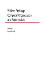
Figure 12.13, is a
simplified diagram of a
16-bit analog to digital
converter. At it’s heart is
a 16-bit D/A converter
and a comparator. The
operation of the circuit
is very straightforward.
We start by applying
the digital code $0000
to the D/A converter.
The output of the D/A
converter is 0 volts. The output is applied to the minus input of the comparator. The voltage that
we want to digitize is applied to the positive input of the comparator. We then add a count of 1 to
the digital code and apply the 16-bit code to the D/A converter. The output voltage will increase
slightly because we have 65,534 codes to go. However, we also check the output of the comparator
to see if it changed from 1 to 0. When the comparator’s output changes state, then we know that
the output voltage of the D/A converter is just slightly greater than the unknown voltage.
When it changes state we stop counting up and the digital code at the time the comparator changes
state is the digital value of the unknown analog voltage. We call this a single-ramp A/D converter
because we increase the test voltage in a linear ramp until the test voltage and the unknown voltage
are equal.
Imagine that you were building a single ramp A/D converter as part of a computer-based data log
-
ging system. You would have a 16-bit I/O port as your digital output port and a single bit (
TEST)

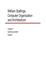
input to sample the state of the comparator output. Starting from an initialized state you would
keep incrementing
the digital code and
sampling the TEST
input until you saw
the TEST input go
low. The flow chart
of this algorithm for
the single ramp A/D
is shown in Figure
12.14.
The single ramp has
the problem that the
digitizing time is
Figure 12.13: A 16-bit, single ramp analog to digital converter.
16-bit D/A Converter
D0
D15
………………
To
I/O Port
Vo
ut
Vx +
–
Comp.
Vo
ut = > Vx
TEST
Figure 12.14: Algorithm for the single ramp A/D converter.

Initialize
COUNT
to zero
Read
TEST
bit
IS
TEST
TRUE
YES
COUNT = Digitized Voltage
NO
Increment
COUNT
Vx
COUNT
0000
FFFF
TEST = TRUE
Interfacing with the Real World
343
variable. A low voltage will digitize quickly, a high voltage will take longer. Also, the algorithm of
the single ramp is analogous to a linear search algorithm. We already known that a binary search is
more efficient than a linear search, so as you might imagine, we could also use this circuit to do a
binary progression to zero in on the unknown voltage. This is called the successive approximation

A/D converter and it is the most commonly used design today.
The algorithm for the successive approximation A/D converter is just as you would expect of a
binary search. Instead of starting at the digital code of 0x0000, we start at 0x8000. We check to see
if the comparator output is 1 or 0, and we either set the next most significant bit to 1 or to 0. Thus,

the 16-bit A/D can determine the unknown voltage in 16 tests, rather than as many as 65,535.
The last type of A/D converter is the voltage to frequency converter, or V/F converter. This con
-
verter converts the input voltage into a stream of digital pulses. The frequency of this pulse stream
is proportional to the analog voltage. For example, a V/F converter can have a transfer function of
10 KHz per volt. So at 1 volt in, it has a frequency output of 10,000 Hertz. At 10 volts input, the
output is 100,000 Hertz, and so on. Since we know how to accurately measure quantities related to
time, it is possible to very accurately measure frequency and count pulses, we are effectively doing
a voltage to time conversion.
The V/F converter has one very attractive feature. It is extremely effective in filtering out noise in
an input signal. Suppose that the output of the V/F converter is around 50,000 Hz. Every second,
the V/F emits approximately 50,000 pulses. If we keep counting and accumulating the count, in
10 seconds we count 500,000 pulses, in 100 seconds we count 5,000,000 pulses, and so forth.
On a finer scale, perhaps each second the count is sometimes slightly greater than 50,000, some
-
times slightly less. The longer we keep counting, the more we are averaging out the noise in our
unknown voltage. Thus, if we are willing to wait long enough, and our input voltage is stable for
that period of time, we can average it to a very high accuracy.
Now that we understand how an analog to digital converter actually works, let’s look at a complete
data logging system that we might use to measure several analog inputs.
Figure 12.15 is a simplified schematic diagram of such a data logger. There are several circuit
elements in Figure 12.15 that we haven’t discussed before. For the purposes of this example it isn’t
necessary to go into a detailed analysis of how they work. We’ll just look at their overall operation
in the context of understanding how the process of data logging takes place.
The block marked ‘Signal Conditioning’ is usually a set of amplifiers or other form of signal con
-
verters. The purpose is to convert the analog signal from the sensor to a voltage that is in the range
of the A/D converter. For example, suppose that we are trying to measure the output signal from a
sensor whose output voltage range is 0 to 1 mV. If we were to feed this signal directly into an A/D
converter with an input range of 0–10 volts, we would never see the output of the sensor. Thus, it

is likely that we would use an analog amplifier to amplify the sensor’s signal from the range of
0 to 0.001 volts to a range of 0 to 10 volts.
Presumably each analog channel has different amplification requirements, so each channel is
handled individually with its own amplifier or other type of signal conditioner. The point is that we
want each channel’s sensor range to be optimally matched to the input range of the A/D converter.
Chapter 12
344
Notice that the data logging system is designed to monitor 8 input channels. We could connect
an A/D converter to each channel, but usually that is not the most economical solution. Another
analog circuit element, called an analog multiplexer, is used to sequentially connect each of the
analog channels to the A/D converter. In a very real sense, the analog multiplexer is like a set of
tri-state output devices connected to a common bus. Only one output at a time is allowed to be
connect to the bus. The difference here is that the analog multiplexer is capable of preserving the
analog voltage of its input signal.
The next device is called a sample and hold module, or
S/H. This takes a bit more explaining to
make sense of. The S/H module allows us to digitize an analog signal that is changing with time.
Previously we saw that it can take a significant amount of time to digitize an analog voltage. A
single-ramp A/D might have to count up several thousand counts before it matched the unknown
voltage. Through all of these examples we always assumed that the unknown analog voltage was
nice and constant. Suppose for a moment that it is the sound of a violin that we are trying to faith-
fully digitize. At some instant of time we want to know a voltage point on the violin’s waveform,
but what is it? If the unknown voltage of the violin changes significantly during the time it takes
the A/D converter to digitize it, then we may have a very large error to deal with. The S/H module
solves this problem.
The S/H module is like a video freeze-frame. When the digital input is in the sample position

(S/H = 1) the analog output follows the digital input. When the S/H input goes low, the analog
voltage is frozen in time, and the A/D converter can have a reasonable chance of accurately digitiz
-

ing it. To see why this is, let’s consider a simple example. Suppose that we are trying to digitize a
sine wave that is oscillating at a frequency of 10 KHz. Assume that the amplitude of the sine wave
is ±5 volts. Thus,
Figure 12.15: Simplified schematic diagram of a computer-based data logger.
Analog input
Channel 1
Analog input
Channel 2
Analog input
Channel 3
Analog input
Channel 4
Analog input
Channel 5
Analog input
Channel 6
Analog input
Channel 7
Analog input
Channel 8
Signal Conditioning
Analog Multiplexer
Sample
and
Hold
S / H
A/D
Converter
Convert
Data ready/EOC

Computer
System
Output Port 0: bit 0
Interrupt input port
Output por
t 0: bit 1
Channel select 0
Channel select 1
Channel select 2
Output por
t 0: bit 2
Output port 0: bit 3
Output port 0: bit 4
8-bit digitized data
Input port 1
D0
D7
Interfacing with the Real World
345
V(t) = 5sin(ωt)
where ω is the angular frequency of the sine wave, measured in radians per second. If this is new
to you, just trust me and go with the flow. The angular frequency is just 2
πf, where f is the actual
frequency of the sine wave in Hertz (cycles per second). The rate of change of the voltage is just
the first derivative of V(t):
dV/dt = –5ωcost(ωt) = –10πfcos(ωt).
The maximum rate of change of the voltage with time occurs when cos(
ωt) = 1, so
dV/dt(maximum) = –10πf or –31.4 × 10x10
3

.
Thus, the maximum rate of change of the voltage with time is 0.314 volts per microsecond. Now,
if our A/D converter requires 5 microseconds to do a single conversion, then the unknown voltage
may change as much as ~1.5 volts during the time the conversion is taking place. Since this is usu-
ally an unacceptable large error source, we need the S/H module to provide a stable signal to the
A/D converter during the time that the conversion is taking place.
We now know enough about the system to see how it functions. Let’s do a step-by-step analysis:
1. Bits 2:4 of output port 0 select the desired analog channel to connect to the S/H module.
2. The conditioned analog voltage appears at the input of the S/H module.
3. Bit 1 of output port 0 goes low and places the S/H module in hold mode. The analog input
voltage to be digitized is now locked at its value the instant of time when S/H went low.
4. Bit 0 of output port 0 issues a positive pulse to the A/D converter to trigger a convert cycle
to take place.
5. After the required conversion interval, the end-of-conversion
signal (EOC) goes low, caus-
ing an interrupt to the computer.
6. The computer goes into its ISR for the A/D converter and reads in the digital data.
7. Depending on its algorithm, it may select another channel and read another input value, or
continue digitizing the same channel as before.
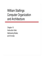
Figure 12.16 summarizes the degree of difficulty required to build an A/D converter of arbitrary
speed and accuracy. The areas labeled “SK”, although theoretically rather straightforward to do,
often require application-specific knowledge. For example, a heart monitor may be relatively slow
and medium accuracy, but the
requirements for electrically pro-
tecting the patient from any shock
hazards may impose addition
requirement for a designer.
Figure 12.16: Graph summarizing
degree of difficulty producing an
A/D converter of a given accuracy

and conversion rate. From Horn
3
.
Conversion Rate
Effective number of bits
SK = Specialized Knowledge
6
8
10
12
14
16
18
20
22
24
26
1 10 100 1K 10K 100K 1M 10M 100M 1G
SK
DIFFICUL
T
DIFFICULT TO
IMPOSSIBLE
FAIRLY
EASY
SK
Chapter 12
346
The Resolution of A/D and D/A Converters
Before we leave the topic of analog-to-digital and digital-to-analog converters we should try

to summarize our discussion of what we mean by the resolution of a converter. The discussion
applies equally to the D/A converter, but is somewhat easier to explain from the perspective of the
A/D converter, so that’s what we’ll do. When we try to convert an analog voltage, or current or
resistance (remember Ohm’s Law?) to a corresponding digital value, we’re faced with a fundamen
-
tal problem. The analog voltage is a continuously variable quantity while the digital value can only
be represented in discrete steps.
You’re already familiar with this problem from your C++ programming classes. You know, or
should know, that certain operations are potentially dangerous because they could result in errone
-
ous results. In programming, we call this a “round-off error”. Consider the following example:
float A = 3.1415906732678;
float B = 3.1415906732566;
if ( A == B)
{do something}
else
{do something else}
What will it do? Unless you knew how many digits of precision you can represent with a float on
your computer, you may or may not get the result you expect. We have the same problem with A/D
converters. Suppose I have a precision voltage source. This is an electronic device that can provide
a very stable voltage for long periods of time. Typically, special batteries, called standard cells,

are used for this. Let’s say that we just spent $500 and sent our standard cell back to the National
Institute for Standards and Testing in Gaithersburg, MD.
After a few weeks we get the standard cell back from NIST with a calibration certificate stating
that the voltage on our standard cell is +1.542324567 volts at 23 degrees, Celsius (there is a slight
voltage versus temperature shift, but we can account for it ). Now we hook this cell up to our A/D
converter and take a reading. What will we measure?
Right now you don’t have enough information to answer that so let’s be a bit more specific:
A/D range: 0 volts – +2.00 volts

A/D resolution: 10 bits
A/D accuracy: +/– 1/2 least significant bit (LSB)
This means that over the analog input range of 0.00 to +2.00 volts, there are 1024 digital codes
available to us to represent the analog voltage. We know that 0.00 volts should give us a digital
value of 00 0000 0000 and that +2.00 volts should give us a digital value of 11 1111 1111, but
what about everything in between? At what point does the digital code change from 0x000 to
0x001? In other words, how sensitive is our A/D converter to changes, or fluctuations, in the ana
-
log input voltage?
Let’s try to figure this out. Since there are 1023 intervals between 0x000 and 0x3FF we can calcu
-
late what interval in the analog voltage corresponds 1 change of the digital voltage.
Interfacing with the Real World
347
Therefore 2.00 / 1023 = 1.9550 × 10
–3

volts. Thus, every time the analog voltage
changes by about 2 millivolts (mV) we
should see that the digital code also chang
-
es by 1 unit. This value of 2 mV is also
what we would call the least significant
bit because this amount of voltage change
would cause the LSB to change by 1.
Consider Figure 12.17. The stair-step
looking curve represents the transfer
function for our A/D converter. It shows
us how the digital code will change as a
function of the analog input voltage. No

-
tice how we get a digital code of 0x000 up
until the analog voltage rises to almost 1
mV. Since the accuracy is 1/2 of the LSB,
we have a range of analog voltage cen
-
tered about each analog interval (vertical dotted lines). This is the region defined by the horizontal
portion of the line. For example, the digital code will be $001 for an analog voltage in the range of
just under 1 mV to just under 3 mV.
What happens if our analog voltage is right at the switching point? Suppose it is just about

0.9775 mV? Will the digital code be $000 or $001? The answer is, “Who knows?” Sometimes it
might digitize as $000 and other times it might digitize as $001.
Now back to our standard cell. Recall that the voltage on our standard cell is +1.542324567 volts.
What would the digital code be? Well +1.542324567 / 1.9550 × 10
–3
= 788.913, which is almost
789. In hexadecimal, 789
10
equals 0x315, so that’s the digital code that we’d probably see.
Is this resolution good enough? That’s a hard question to answer unless we know the context of
the question. Suppose that we’re given the task of writing a software package that will be used
to control a furnace in a manufacturing plant. The process that takes place in this furnace is quite
sensitive to temperature fluctuations, so we must exhibit very tight control. That is, the temperature
must be held at exactly 400 degrees Celsius, +/– 0.1 degree Celsius. Now the temperature in the
furnace is being monitored by a thermocouple whose voltage output is measured as follows:
Voltage output @ 400 degrees Celsius = 85.000 mV
Transfer function = .02 mV / degree Celsius
so far, this doesn’t look too promising. But we can do some things to improve the situation. The
first thing we can do is amplify the very low level voltages output by the thermocouple and raise it

to something more manageable. If we use an amplifier that can amplify the input voltage by a fac
-
tor of 20 times (gain = 20 ) then our analog signal becomes:
Voltage output @ 400 degrees Celsius ( X 20 ) = 1.7000 V
Transfer function ( X 20 ) = .4 mV / degree Celsius
Figure 12.17: Transfer function for a 10-bit A/D converter
over a range of 0 to 2.00 volts. Accuracy is 1/2 LSB.
011
010
001
000
Analog Voltage (mV)
0 1 2 3 4
Digital Code
Chapter 12
348
Now the analog voltage range is OK. Our signal is 1.7 volts at 400 degrees Celsius. This is less than
the 2.00 maximum voltage of the A/D converter, so we’re not in any danger of going off scale. What
about our resolution? We know that our analog signal can vary over a range of almost 2 mV before
the A/D converter will detect a change. Referring back to the specifications for our amplified ther
-
mocouple, this means that the temperature could shift by about 5 degrees Celsius before the

A/D converter could detect a variation. Since we need to control the system to better than 0.1
degree, we need to use an A/D converter with better resolution. How much better? Well, we would
predict that a change in the temperature of 0.1 degree Celsius would cause a voltage change of

0.04 mV. Therefore, we’ve got to improve our resolution by a factor of 2 mV / 0.04 mV or 50 times!
Is this possible? Let’s see. Suppose we decided to sell our 10-bit A/D converter on eBay and use
the proceeds to buy a new one. How about a 12-bit converter? That would give us 4096 digital

codes. Going from 1024 codes to 4096 codes is only a 4× improvement in resolution. We need
50X. A 16-bit A/D converter gives us 65,536 codes. This is a 64× improvement. That should work
just fine! Now, we have:
A/D range: 0 volts – +2.00 volts
A/D resolution: 16 bits
A/D accuracy: +/– 1/2 least significant bit (LSB)
Our analog resolution is now 2.00 volts / 65,535 or 0.03 mV per digital code step. Since we need
to be able to detect a change of 0.04 mV, this new converter should do the job for us.
Summary of Chapter 12
Chapter 12 covered:
• The concepts of interrupts as a method of dealing with asynchronous events,
• How a computer system deals with the outside world through I/O ports
• How physical quantities in the real world events are converted to a computer-compatible
format and vice versa through the processes of analog-to-digital conversion and digital-to-
analog conversion.
• The need for an analog to digital interface device called a comparator.
• How Ohm’s Law is used to establish fixed voltage points for A/D and D/A conversion.
• The different types of A/D converters and their advantages and disadvantages.
• How accuracy and resolution impact the A/D conversion process.
Chapter 12: Endnotes
1
Glenn E. Reeves, “Priority Inversion: How We Found It, How We Fixed It,” Dr. Dobb’s Journal, November, 1999, p. 21.
2
Arnold S. Berger, A Brief Introduction to Embedded Systems with a Focus on Y2K Issues, Presented at the Electric
Power Research Institute Workshop on the Year 2000 Problem in Embedded Systems, August 24–27, 1998,

San Diego, CA.
3
Jerry Horn, High-Performance Mixed-Signal Design, />349
1. Write a subroutine in Motorola 68000 assembly language that will enable a serial UART

device to transmit a string of ASCII characters according to the following specification:
a. The UART is memory mapped at byte address locations $2000 and $2001.
b. Writing a byte of data to address $2000 will automatically start the data transmission pro-
cess and it will set the Transmitter Buffer Empty Flag (TBMT) in the STATUS register to 0.
c. When the data byte has been sent, the TBMT flag automatically returns to 1, indicating
that TBMT is TRUE.
d. The STATUS register is memory mapped at byte address $2001. It is a READ ONLY
register and the only bit of interest to you is DB0, the TBMT flag.
e. The memory address of the string to be transmitted is passed into the subroutine in
register A6.
f. The subroutine does not return any values.
g. All registers used inside the subroutine must be saved on entry and restored on return.
h. All strings consist of the printable ASCII character set, 00 thru $7F, located in successive
memory locations and the string is terminated by $FF.
The UART is shown schematically in the figure shown below:
Notes:
• Remember, you are only writing a subrou-
tine. There is no need to add the pseudo-ops
that you would also add for a program.
• You may assume that the stack is already
defined.
• You may use EQUates in your program
source code to take advantage of symbolic
names.
2. Examine the block of 68K assembly language code shown below. There is a serious error in
the code. Also shown is the content of the first 32-bytes memory.
a. What is the bug in the code?
b. What will the processor do when the error occurs? Explain as completely as possible,
given the information that you have.
Exercises for Chapter 12

DATA REGISTER
Shift out
STATUS REGISTER
Memor
y address $2000
Memory address $2001
TB = TBMT FLAG
X = Don’t care
DB7 DB0
DB7 DB0
x x x x x x x TB
Chapter 12
350
org $400
start lea $2000,A0
move.l #$00001000,D0
move.l #$0000010,D1
loop divu D1,D0
move.l D0,(A0)+
subq.b #08,D1
bpl loop
end $400
Memory contents (Partial)
00000000 00 00 A0 00 00 00 04 00 00 AA 00 00 00 AA 00 00
00000010 00 AA 00 00 00 CC AA 00 00 AA 00 00 00 AA 00 00
Note: The first few vectors of the Exception Vector Table are listed below:
Vector # Memory Address Description
0 $00000000 RESET: supervisor stack pointer
1 $00000004 RESET: program counter
2 $00000008 Bus Error

3 $0000000C Address Error
4 $00000010 Illegal instruction
5 $00000014 Zero Divide
6 $00000018 CHK Instruction
7 $0000001C TRAPV instruction
8 $00000020 Privilege violation
3. Assume that you have two analog-to-digital converters as shown in the table, below:
Converter type Resolution (bits) Clock rate (MHz) Range (volts)
Single Ramp 16 1.00 0 to +6.5535
Successive Approximation 16 1.00 0 to +6.5535
How long (time in microseconds) will it take each type of converter to digitize an analog volt-
age of +1.5001 volts?
4. Assume that you may assign a priority level from 0 (lowest) to 7 (highest, NMI ) for each of
the following processor interrupt events. For each of the following events, assign it a priority
level and briefly describe your reason for assigning it that level.
a. Keyboard strike input.
b. Imminent Power failure.
c. Watchdog timer.
d. MODEM has data available for reading.
e. A/D converter has new data available.
f. 10 millisecond real time clock tick.
g. Mouse click.
h. Robot hand has touched solid surface.
i. Memory parity error.
Interfacing with the Real World
351
5. Assume that you have an 11-bit A/D converter that can digitize an analog voltage over the
range of –10.28V to + 10.27volts. The output of the A/D converter is formatted as a 2’s com
-
plement positive or negative number, depending upon the polarity of the analog input signal.

a. What is the minimum voltage that an analog input voltage could change and be guaran
-
teed to be detected by a change in the digital output value?
b. What is the binary number that represents an analog voltage of –5.11 volts?
c. Suppose that the A/D converter is connected to a microprocessor with a 16-bit wide data
bus. What would the hexadecimal number be for an analog voltage of +8.96V? Hint: It is
not necessary to do any rescaling of the 11-bit number to 16-bits.
d. Assume that the A/D converter is a successive approximation-type A/D converter. How
many samples must it take before it finally digitizes the analog voltage?
e. Suppose that the A/D converter is being controlled by a 1 MHz clock signal and a sample
occurs on the rising edge of every clock. How long will it take to digitize an analog voltage?
6. Assume that you are the lead software designer for a medical electronics company. Your new
project is to design the some of the key algorithms for a line of portable heart monitors. In
order to test some of your algorithms you set up a simple experiment with some of the prelimi
-
nary hardware. The monitor will use a 10-bit analog to digital converter (A/D) with an input
range of 0 to 10 volts. An input voltage of 0 volts results in a binary output of 0000000000 and
an input voltage of 10 volts results in a binary output of 1111111111. It digitizes the analog
signal every 200 microseconds. You decide to take some data. Shown below is a list of the
digitized data values (in hex).
2C8, 33B, 398, 3DA, 3FC, 3FB, 3D7, 393, 334, 2BF, 23E, 1B8, 137, 0C4, 067, 025, 003, 004,
028, 06C, 0CB, 140, 1C1, 247
Once you collect the data you want to write it out to a strip chart meter and display it so a
doctor can read it. The strip chart meter has an input range of –2 volts to +2 volts. Fortunately,
your hardware engineer has designed a 10-bit digital to analog (D/A) circuit such that a binary
digital input value of 0000000000 cause an analog output of –2 volts and 1111111111 causes
an output of +2 volts. You write a simple algorithm that sends the digitized data to the chart so
you can see if everything is working properly.
a. Show what the chart recorder would output by plotting the above data set on graph paper.
b. Is there any periodicity to the waveform? If so, what is the period and frequency of the

waveform?
7. Suppose that you have a 14-bit, successive approximation, A/D converter with a conversion
time of 25 microseconds.
a. What is the maximum frequency of an AC waveform that you can measure, assuming that
you want to collect a minimum of 4 samples per cycle of the unknown waveform?
b. Suppose that the converter can convert an input voltage over the range of –5V to +5V,
what is the minimum voltage change that should be measurable by this converter?
c. Suppose that you want to use this A/D converter with a particular sample and hold circuit
(S/H) that has a droop rate of 1 volt per millisecond. Is this particular S/H circuit compat-
ible with the A/D converter? If not, why?
Chapter 12
352
8. Match the applications with the best A/D converter for the job. The converters are listed below:
A. 28-bit successive approximation A/D converter, 2 samples per second
B. 12-bit, successive approximation A/D, 20 microsecond conversion time.
C. 0 – 10 KHz voltage to frequency converter, 0.005% accuracy.
D. 8-bit flash converter, 20 nanosecond conversion time.
a. Artillery shell shock wave measurements at an Army research lab. ______
b. General purpose data logger for weather telemetry.______
c. 7-digit laboratory quality digital voltmeter.______
d. Molten steel temperature controller in a foundry.______
9. Below is a list of “C” function prototypes. Arrange them in the correct order to interface your
embedded processor to an 8-channel 12-bit A/D converter system.
a. boolean Wait( int ) /* True = done, int defines # of */
/* milliseconds to wait before timeout */
b. int GetData ( void ) /* Returns the digitized data value */
c. int ConfidenceCheck( void ) /* Perform a confidence check on the */
/* hardware */
d. void Digitize( void ) /* Turn on A/D converter to digitize */
e. void SelectChannel( int ) /* Select analog input channel to read */

f. void InitializeHardware( void ) /* Initialize the state of the hardware to a */
/* known condition */
g. void SampleHold( boolean ) /* True = sample, False = hold */
10. Assume that you have 16-bit D/A converter, similar in design to the one shown in

Figure 12.12. The current source for the least significant data bit, D0, produces a current of

0.1 microamperes. What is the value of the resistor needed so that the full scale output of the
D/A converter is 10.00 volts?
353
C H A P T E R
13
Introduction to Modern
Computer Architectures
Objectives
When you are finished with this lesson, you will be able to:
 Describe the basic properties of CISC and RISC architectures;
 Explain why pipelines are used in modern computers;
 Explain the advantages of pipelines and the performance issues they create;
 Describe how processors can execute more than one instruction per clock cycle;
 Explain methods used by compilers to take advantage of a computer’s architecture in
order to improve overall performance.
Today, microprocessors span a wide range of speed, power, functionality and cost. You can pay
less than 25 cents for a 4-bit microcontroller to over $10,000 for a space-qualified custom proces
-
sor. There are over 300 different types of microprocessors in use today. How do we differentiate
among such a variety of computing devices? Also, for the purposes of this text we will not con
-
sider mainframe computers (IBM, VAX, Cray, Thinking Machines, and so forth), but rather, we’ll
confine our discussion to the world of the microprocessor.

There are three main microprocessor architectures in general use today. These are:
CISC, RISC,
DSP. We’ll discuss what the acronyms stand for in a little while, but for now, how do we differenti
-
ate among these multiple devices? What factors identify or differentiate the various families? Let’s
first try to identify the various ways that we can rack and stack the various configurations.
1. Clock speed: Processors today may run at clock speeds from essentially zero, to multiple
gigahertz. With modern CMOS circuit design, the amount of power a device consumes is
generally proportional to its clock frequency. If you want a microprocessor to last 2 years
running on an AAA battery on the back of a whale, then don’t run the clock very fast, or
better yet, don’t run it at all, but wake up the processor every so often to do something use
-
ful and then let it go back to sleep.
2. Bus width: We can also differentiate processors by their data path width: 4, 8, 16, 32, 64,
VLIW (very long instruction word). In general, if you double the width of the bus, you can
roughly speed-up the processing of an algorithm between 2 and 4 times.
3. Processors have varying amounts of addressable address space, from 1 Kbyte for a simple
microcontroller to multi-gigabyte addressing capabilities in the Pentium, SPARC, Athlon
and Itanium class machines. A PowerPC processor from Freescale has 64-bit memory
addressing capabilities.
Chapter 13
354
4. Microcontroller/Microprocessor/ASIC: Is the device strictly a CPU, such as a Pentium or
Athlon? Is it an integrated CPU with peripheral devices, such as a 68360? Or is it a library
of encrypted Verilog or VHDL code, such as an ARM7TDMI, that will ultimately be
destined for a custom integrated circuit design?
As you’ve seen, we can also differentiate among processors by their instruction set architectures
(ISA). From a software developer’s perspective, this is the architecture of a processor and the dif-
ferences between the ISA’s determine the usefulness of a particular architecture for the intended
application. In this text we’ve studied the Motorola 68K ISA, the Intel x86 and the ARM v4 ISAs,

but they are only three of many different ISA’s in use today. Other examples are 29K, PPC, SH,
MIPS and various DSP ISA’s. Even within one ISA we can have over 100 unique microproces
-
sors or integrated device. For example, Motorola’s microprocessor family is designated by 680X0,
where the X substitutes for the numbers of various family members. If we take the microproces
-
sor core of the 68000 and add some peripheral devices to it, it becomes the 6830X family. Other
companies have similar device strategies.
Modern processors also span a wide range of clock speeds, from 1MHz or less, to over 3 GHz
(3000 MHz). Not too long ago, the CRAY supercomputer cost over $1M and could reach the
unheard of clock speed of 1 GHz. In order to achieve those speeds the engineers at CRAY had to
construct exotic, liquid cooled circuit boards and control signal timing by the length of the cables
that carried them. Today, most of us have that kind of performance on our desktop. In fact, I’m
writing this text on a PC with a 2.0 GHz AMD Athlon processor that is now consider to be third
generation by AMD. Perhaps if this text is really successful, I can use my royalty checks to up
-
grade my PC to an Athlon™ 64. Sigh…
Processor Architectures, CISC, RISC and DSP
The 68K processor and its instruction set, the 8086 processor and its instruction set are examples
of the complex instruction set computer (CISC), architecture. CISC is characterized by having
many instructions and many addressing modes. You’ve certainly seen for yourself many assembly
language instructions and variations on those instructions we have. Also, these instructions could
vary greatly in the number of clock cycles that one instruction might need to execute. Recall, the
table shown below. The number of clock cycles to execute a single instruction varied from 8 to 28,
depending upon the type of MOVE being executed.
Instruction Clock Cycles Instruction Time (usec)*
MOVE.B #$FF,$1000 28 1.75
MOVE.B D0,$1000 20 1.25
MOVE.B D0,(A0) 12 0.75
MOVE.B D0,(A0)+ 8 0.50

* Assuming a 16 MHz clock frequency
Having variable length instruction times is also characteristic of CISC architectures. The CISC
instruction set can be very compact because these complex instructions can each do multiple
operations. Recall the DBcc, or the test condition, decrement and branch on condition code
instruction. This is a classic example of a CISC instruction. The CISC architecture is also called
Introduction to Modern Computer Architectures
355
the von Neumann architecture, after John von Neumann, who is credited with first describing the
design that bears his name. We’ll look at an aspect of the Von Neumann architecture in a moment.
CISC processors have typically required a large amount of circuitry, or a large amount of area on
the silicon integrated circuit die. This has created two problems for companies trying to advance
the CISC technology: higher cost and slower clock speeds. Higher costs can result because the
price of an integrated circuit is largely determined the fabrication yield. This is a measure of how
many good chips (yield) can be harvested from each silicon wafer that goes through the IC fabrica
-
tion process. Large chips, containing complex circuitry, have lower yields than smaller chips. Also,
complex chips are difficult to speed up because distributing and synchronizing the clock over the
entire area of the chip becomes a difficult engineering task.
A computer with a von Neumann architecture has a single memory space that contains both the
instructions and the data, see Figure 13.1 The CISC computer has a single set of busses linking the
CPU and memory. Instructions and data must share the same path to the CPU from memory, so if
the CPU is writing a data value
out to memory, it cannot fetch the
next instruction to be executed. It
must wait until the data has been
written before proceeding. This is
called the von Neumann bottle-
neck
because it places a limitation
on how fast the processor can run.

Howard Aiken of Harvard Uni
-
versity invented the Harvard
architecture (he must have been
too modest to place his name
on it). The Harvard architecture
features a separate instruction
memory and data memory. With
this type of a design, both data
and instructions could be operated on independently. Another subtle difference between the von
Neumann and Harvard architectures is that the von Neumann architecture permits self-modifying
programs, the Harvard architecture does not. Since the same memory space in the von Neumann
architecture may hold data and program code, it is possible for an instruction to change the in-
struction in another portion of the code space. In the Harvard Architecture, loads and stores can
only occur in the data memory, so
self-modifying code is much harder to do.
The Harvard architecture is generally associated with the idea of
a reduced instruction set com-
puter, or
RISC, architecture, but you can certainly design a CISC computer with the Harvard
Architecture. In fact, it is quite common today to have CISC architectures with separate on-chip
cache memories for instructions and data.
The Harvard architecture was used commercially on the Am29000 RISC microprocessor, from
Advanced Micro Devices (AMD). While the Am29K processor was used commercially in the first
Figure 13.1: Memory architecture for the von Neumann (CISC)
and Harvard (RISC) architectures.
von Neumann
CPU
Memory
Instructions

Data
von Neumann
“bottleneck”
von Neumann
“bottleneck”
Harvard
CPU
Instruction
Memory
Data
Memory
Address,
Data and
Status
Busses
Data space
Address
,
Data and
Status
Busses
Instruction
Address,
Data and
Status
Busses
Chapter 13
356
LaserJet series of printers from Hewlett-Packard, designers soon complained to AMD that
29K-based designs were too costly because of the need to design two completely independent

memory spaces. In response, AMD’s follow-on processors all used a single memory space for
instructions and data, thus forgoing the advantages of the Harvard architecture. However, as we’ll
soon see, the Harvard architecture lives on in the inclusion of on-chip instruction and data caches
in many modern microprocessors. Today, you can design ARM processor implementations with
either a von Neumann or Harvard architecture.
In the early 1980’s a number of researchers were investigating the possibility of advancing the
state of the art by streamlining the microprocessor rather than continuing the spiral of more and
more complexity
1,2
. According to Resnick
3
, Thornton
4
explored aspects of certain aspects of the
RISC architecture in the design of the CDC 6600 computer in the late 60’s. Among the early
research carried out by the computer scientists who were involved with the development of the
RISC computer were studies concerned with what fraction of the instruction sets were actually
being used by compiler designers and high-level languages. In one study
5
the researchers found
that 10 instructions accounted for 80% of all the instructions executed and only 30 instructions
accounted for 99% of all the executed instructions. Thus, what the researchers found was that most
of the time, only a fraction of the instructions and addressing modes were actually being used.
Until then, the breadth and complexity of the ISA was a point of pride among CPU designers; sort
of a “My instruction set is bigger than your instruction set” rivalry developed.
In the introductory paragraph to their paper, Patterson and Ditzel note that,
Presumably this additional complexity has a positive tradeoff with regard to the cost-
effectiveness of newer models. In this paper we propose that this trend is not always
cost-effective, and in fact, may even do more harm than good. We shall examine the case
for a Reduced Instruction Set Computer (RISC) being as cost-effective as a Complex

Instruction Set Computer (CISC).
In their quest to create more and more complex and elegant instructions and addressing modes, the
CPU designers were creating more and more complex CPUs that were becoming choked by their
own complexity. The scientists asked the question, “Suppose we do away with all but the most
necessary instructions and addressing modes. Could the resultant simplicity outweigh the inevi
-
table increase in program size?”
The answer was a resounding, “Yes!” Today RISC is the dominant architecture because the gains
over CISC were so dramatic that even the growth in code size of 1.5 to 2 times was far outweighed
by the speed improvement and overall streamlining of the design. Today, a modern RISC processor
can execute more than one instruction per clock cycle. This is called a superscalar architecture.

When we look at pipelines, we’ll see how this dramatic improvement is possible. The original
RISC designs used the Harvard architecture, but as caches grew in size, they all settled on a single
external memory space.
However, everything isn’t as simple as that. The ISA’s of some modern RISC designs, like the
PowerPC, has become every bit as complex as the CISC processor it was designed to improve
upon. Also, aspects of the CISC and RISC architectures have been morphing together, so drawing
distinctions between them is becoming more problematic. For example, the modern Pentium and
Introduction to Modern Computer Architectures
357
Athlon CPUs execute an ISA that has evolved from Intel’s classic x86, CISC architecture. How-
ever, internally, the processors exhibit architectural features that would be characteristic of a RISC
processor. Also, the drive for speed has been led by Intel and AMD, and today’s 3+ gigahertz
processors are the Athlons and Pentiums.
Both CISC and RISC can get the job done. Although RISC processors are very fast and efficient,
the executable code images for RISC processors tend to be larger because there are fewer instruc
-
tions available to the compiler. Although this distinction is fading fast, CISC computers still tend
to be prevalent in control applications, such as industrial controllers, instrument controllers.

On the other hand, RISC computers tend to prevail in data processing applications where the focus
of the algorithm is
Data in >>> Do some processing >>> Data out.
The RISC processor, because of its simplified instruction set and high speed, is well suited for
algorithms that stress data movement, such as might be used in telecommunications or games.
The digital signal processor (DSP) is a specialized type of mathematical data processing com-
puter. DSPs do math instead of control (CISC) or data manipulation (RISC). Traditionally, DSP
were classic CISC processors with several architectural enhancements to speed-up the execution of
special categories of mathematical operations. These additions were circuit elements such as barrel
shifters and multiply/accumulate (MAC) instructions (See figure 11.2) that we looked at when we
examined the ARM multiplier block. Recall, for example, the execution of an inner loop:
• fetch an X constant and a Y variable
• multiply them together and accumulate (SUM) the result
• check if loop is finished
The DSP accomplished in one instruction what a CISC processor took eight or more instructions to
accomplish. Recall from integral calculus that calculating the integral of a function is the same as
calculating the area under the curve of that function. We can solve for the area under the curve by
multiplying the height at each point by the width of a small rectangular approximation under the
curve and the sum the area of all of these individual rectangles. This is the MAC instruction in a DSP.
The solution of integrals is an important part of solving many mathematical equations and trans
-
forming real time data. The domain of the DSP is to accept a stream of input data from an A/D
converter operate on it and output the result to a D/A converter. Figure 13.2 shows a continuously
varying signal going into the DSP
from the A/D converter and the
output of the DSP going to a D/A
converter. The DSP is processing the
data stream in real time. The analog
data is converted to its digital repre
-

sentation and then reconverted to analog after processing.
Several “killer apps” have emerged for the DSP. The first two were the PC modem and PC sound
card. Prior to the arrival of the PC, DSP were special use devices, mostly confined to military
and CIA types of applications. If you’ve ever participated in a conference call and spoken on a
Figure 13.2: Continuous data processing in a DSP.
Continuously
va
rying
signal
Continuously
va
rying
signal
A/D
Conversion
Digital
Signal
Processing
D/A
Conversion
Chapter 13
358
speakerphone, you’ve had your phone conversation processed by a DSP. Without the DSP, you
would get the annoying echo and screech effect of feedback. The DSP implements an echo cancel
-
lation algorithm that removes the audio feedback from your conversation as you are speaking in
real time. The newest application of the DSP in our daily lives is the digital camera. These devices
contain highly sophisticated DSP processors that can process a 3 to 8 megapixel image, converting
the raw pixel data to a compress jpeg image, in just a few seconds.
An Overview of Pipelining

We’ll need to return to our discussion of CISC and RISC in a little while because it is an important
element of the topic of pipelining. However, first we need to discuss what we mean by pipelining.
In a sense, pipelining in a computer is a necessary evil. According to Turley
6
:
Processors have a lot to do and most of them can’t get it all done in a single clock cycle.
There’s fetching instructions from memory, decoding them, loading or storing operands
and results, and actually executing the shift, add, multiply, or whatever the program calls
for. Slowing down the CPU clock until it can accomplish all this in one cycle is an option,
but nobody likes slow clock rates. A pipeline is a compromise between the amount of work
a CPU has to do and the amount of time it has to do it.
Let’s consider this a bit more deeply. Recall that our logic gates, AND, OR, NOT, and the larger
circuit blocks built from them, are electronic circuits that take a finite amount of time for a signal
to propagate through from input to output. The more gates a signal has to go through, the longer
the propagation delay in the circuit.
Consider Figure 13.3. Here’s a complex functional
block with 8 inputs and 3 outputs. We can assume that
it does some type of byte processing. Assume that each
functional block in the circuit has a propagation delay of
X nanoseconds. The blocks can be simple gates, or more
complex functions, but for simplicity, each block has the
same propagation delay through it.
Also, let’s assume that an analysis of the circuit shows
that the path from input b through to output Z is the longest path in the circuit. In other words, in-
put b must pass through N gates on its way to output Z. Thus, whatever happens when a set of new
inputs appear on a through h we have to wait until input b finally ripples through to output Z we
can consider the circuit to have stabilized and that the output data on X, Y
and Z to be correct.
If each functional block has a propagation delay of X ns, then the worst case propagation delay
through this circuit is N*X nanoseconds. Let’s put some real numbers in here. Assume that

X = 300 picoseconds (300x10
-12
seconds) and N = 6. The propagation delay is 1800 picoseconds
(1800 ps). If this circuit is part of a synchronous digital system being driven by a clock, and we
expect that this circuit will do its job within one clock cycle, then the maximum clock rate that we
can have in this system is (1/1800 ps) = 556 MHz.
Keep in mind that the maximum speed that entire computer can run at will be determined by this
one circuit path. How can we speed it up? We have several choices:
Figure 13.3: Propagation delay through a
series of functional blocks.
a
b
c
d
e
f
g
h
X
Y
Z
Block
1
Block
2
Block
N-1
Block
N

Tp = X ns
•
•
•
•
Introduction to Modern Computer Architectures
359
1. Reduce the propagation delay by going to a faster IC fabrication process,
2. Reduce the number of gates that the signal must propagate through,
3. Fire your hardware designers and hire a new batch with better design skills,
4. Pipeline the process.
All of the above options are
usually considered, but the
generally accepted solution by
the engineering team is #4, while
upper management usually favors
option #3. Let’s look at #4 for a
moment. Consider Figure 13.4
Now, each stage of the system
only has a propagation delay of
3 blocks, or 900 ps, for the entire
block. To be sure, we also have
to add in the propagation delay of
the ‘D’ type register, but that’s part of the overhead of the compromise. Assume that at time,

t = 0, there is a rising clock edge and the data is presented to the inputs a through h. After, 900 ps,
the intermediate results have stabilized and appear on the inputs to the first D register, on its in
-
puts, D0 through D10. After any time greater than 900 ps, a clock may come along again and, after
a suitable propagation delay through the register, the intermediate results will appear on the

Q0
through Q10 outputs of the first D register. Now, the data can propagate through the second stage
and after a total time delay of 900 ps + t
p
(register), the data is stable on the inputs to the second D
register. At the next clock rising edge the data is transferred to the second D register and the final
output of the circuit appears on the outputs X,Y and Z.
Let’s simplify the example a bit and assume that the propagation delay through the D register is
zero, so we only need to consider the functional blocks in stages #1 and #2. It still takes a total of
1800 picoseconds for any new data to make it through both stages of the pipeline and appear on
the outputs. However, there’s a big difference. On each rising edge of the clock we can present
new input data to the first stage and because we are using the D registers for intermediate storage
and synchronization, the second stage can still be processing the original input variables while the
first stage is processing new information.
Thus, even though it still takes the same amount of time to completely process the first data,
through the pipeline, which in this example is two clock cycles, every subsequent result (X, Y and
Z) will appear at intervals of 1 clock cycle, not two.
The ARM instruction set architecture that we studied in Chapter 11 is closely associated with the
ARM7TDMI core. This CPU design has a 3-stage pipeline. The ARM9 has a 5-stage pipeline.
This is shown in Figure 13.5.
In the fetch stage the instruction is retrieved from memory. In the decode stage, the 32-bit
instruction word is decoded and the instruction sequence is determined. In the execute stage
the
instruction is carried out and any results are written back to the registers. The ARM9TDMI core
Figure 13.4: A two stage implementation of the digital circuit.
The propagation delay through each stage has been reduced
from 6 to 3 gate delays.
3
STAGE #1
2

1
5
6
STAGE #2
4
D register
D0
D1
D2
D3
D4
D5
D6
D7
D8
D9
D10
Q0
Q1
Q2
Q3
Q4
Q5
Q6
Q7
Q8
Q9
Q10
D register
D0

D1
D2
D3
D4
D5
D6
D7
D8
D9
D10
Q0
Q1
Q2
Q3
Q4
Q5
Q6
Q7
Q8
Q9
Q10
X
Y
Z
a
b
c
d
e
f

g
h
Clock in
Chapter 13
360
uses a 5-stage pipeline. The two ad-
ditional stages, Memory and Write
allow the ARM9 architecture to have
approximately 13% better instruc-
tion throughput than the ARM7
architecture
7
. The reason for this is
illustrates the advantage of a multi-
stage pipeline design. In the ARM7,
the Execute Stage does up to three
operations:
1. Read the source registers,
2. Execute the instruction,
3. Write the result back to the registers.
In the ARM7 design, the registers are read during the decode stage. The execute stage only does
instruction execution, and the Write Stage handles the write-back to the destination register. The
memory stage is unique to the ARM9 and doesn’t have an analog in the ARM7. The ARM7 sup
-
ports a single memory space, holding instructions and data. When, it is fetching a new instruction,
it cannot be loading or storing to memory. Thus, the pipeline must wait (stall) until either the load/
store or instruction fetch is completed. This is the von Neumann bottleneck. The ARM9 uses a
separate data and instruction memory model. During the Memory Stage, load/stores can take place
simultaneously with the instruction fetch in stage 1.
Up to now, everything about the pipeline seemed made for speed. All we need to do to speed up

the processor is to make each stage of the pipeline have finer granularity and we can rev up the
clock rate. However, there is a dark side to this process. In fact, there are a number of potential
hazards to making the pipeline work to its maximum efficiency. In the ARM7 architecture, when
a branch instruction occurs, and the branch is taken, what do we do? There are two instructions
stacked-up behind the branch instruction in the pipeline and suddenly, they are worthless. In other
words, we must flush the pipe and start to refill it again from the memory location of the target of
the branch instruction.
Recall Figure 13.4. It took two clock cycles for the first new data to start exiting the pipeline. Sup
-
pose that our pipeline is a 3-stage design, like the ARM7. It will take 3 clocks for the target of the
branch instruction to make it down the pipe to completion. These additional clocks are extra cycles
that diminish the throughput every time a branch is taken. Since most programs take a branch of
some kind, on average, every 5 to 7 instructions, things can get very slow if we are doing a lot of
branching. Now, consider the situation with a 7 or 9-stage pipeline. Every nonsequential instruc-
tion fetch is a potential roadblock to efficient code flow through the processor.
Later in this chapter we’ll discuss some methods of mitigating this problem, but for now, let’s just
be aware that the pipeline architecture is not all that you might believe it to be. Finally, we need
to cover few odds and ends before we move on. First, it is important to note that the pipeline does
not have to be clocked with exactly the same clock frequency as the entire CPU. In other words,
we could use a frequency divider circuit to create a clock that is ¼ of that of the system clock.
Figure 13.5: Pipeline architectures for the ARM7 and ARM9
CPU core designs.
Fetch
Decode
Execute
Case 1
ARM7
Case 2
Fetch
Decode

Execute
Memory
Write
ARM9
Introduction to Modern Computer Architectures
361
We might then use this slower clock to clock the pipeline, while the faster clock provides us with
a mechanism to implement smaller state machines within each stage of the pipeline. Also, it is
possible that certain stages might cause the pipeline to stall and just mark time during the regular
course of program execution. Load or store to external memory, or instruction fetches will general
-
ly take longer than internal operations, so there could easily be a one or two clock cycle stall every
time there is an external memory operation.
Let’s return to our study of comparative architectures and look at a simpler, nonpipelined
architecture. First we need to appreciate that a processor is an expensive resource, and, just like
expensive machinery, want to always keep it busy. An idle processor is wasting space, energy,
time, etc. What we need is a way to increase performance. In order to understand the problem, let’s
look at how a processor, like the 68K, might execute a simple memory-resident instruction, such
as MOVE.W $XXXX,$YYYY.
According to the 68K Programmer’s Manual, this MOVE.W instruction requires 40 clock cycles
to execute. The minimum 68K instruction time requires seven clock cycles. Where is all this time
being used up?
A new instruction fetch cycle begins when the contents of the PC are transferred to the address
lines. Several cycles are required as the memory responds with the instruction op-code word.
1. The instruction op-code is decoded by the processor.
2. Time is required as the processor generates the first operand (source address) from memory.
3. Time is required to fetch the source data from memory.
4. Time is required to fetch the second operand (destination address) from memory.
5. Time is required to write the data to the destination address.
While all this activity is going on, most of the other functional blocks in the processor are sitting

idle. Thus, another of the potential advantages of pipelining is to break up these execution tasks
Figure 13.6: Execution process for a 68K MOVE instruction.
TIME
ADDRESS
ADDRESS
WAIT
DECODE
DECODE
ADDRESS
ADDRESS
WAIT
EXECUTE
EXECUTE
WAIT
INSTRUCTION EXECUTION TIME
Time required to generate the instruction addres
s
Time required to fetch the instruction from memor
y
Time required to decode the Op Code
Time required to generate the operand addres
s
Time required to fetch the operand
from memor
y
Time required to execute
the instructio
n
Time required to
put away the resul

t
Chapter 13
362
into smaller tasks (stages) so that all of the available resources in the CPU are being utilized to the
greatest extent possible. This is exactly the same idea as building a car on an assembly line. The
overall time to execute one instruction will generally take the same amount of time, but we don’t
need to wait the entire 40 clock cycles for the next instruction to come down the pipe. As we’ve
seen with the ARM processor, and assuming that we didn’t flush the pipe, the next instruction only
needs to go through last stage to finish one stage behind. What we have improved is the throughput
of the system.
In Figure 13.7 we see that
if it takes us two hours to
do a load of laundry, which
includes four tasks (wash
-
ing, drying folding and
putting away), then it would
take eight hours to do four
loads of laundry if they’re
done serially. However, if
we overlap the tasks such
that the next wash load is
started as soon as the first
wash is completed, then we
can complete the entire four
loads of laundry in three and
a half hours instead of eight.
The execution of an instruction is a good example of a physical process with logical steps that can
be divided into a series of finer steps. Let’s look at an example of a three-stage process:
1. Do the first thing. . . .

2. Do the second thing. . . .
3. Do the third thing. . . .
4. Release result. . . .
5. Go back to step #1.
With pipelining, this becomes:
1. Do the first thing, hold the result for step #2.
2. Get the result from step #1 and do the second thing, hold the result for step #3.
3. Get the result from step #2 and do the third thing.
4. Release result.
5. Go back to step #1.
Now, let’s look at the pipelined execution of the 3-stage processes, shown in Figure 13.8. Presum
-
ably, we can create a pipeline because the hardware in Stage #1 becomes idle after executing its
task. Thus, we can start another task in Stage #1 before the entire process is completed. The time
for the first result to exit the pipe is called the flowthrough time.
The time for the pipe to produce
subsequent results is called the clock cycle time.
• Doing tasks serially
• Total time to do 4 laundry loads
T
Total
= 4 × T
A
Pipelining:
When the first resource used by task A is free
(washing machine) begin task B
Time
Task
order
6 PM 7 8 9 10 11 12 1 2 AM

A
B
C
D
Time
6 PM 7 8 9 10 11 12 1 2 AM
Task
order
A
B
C
D
Figure 13.7: Doing the laundry: An example of serial task execution
versus overlapping task. From Patterson and Hennessy
8
.
Introduction to Modern Computer Architectures
363
We see that for the pipe-
line process, it takes a total
time of 5xT
S
to process
3 instructions. Without a
pipeline, the 3 instructions,
executed serially, would
take 9xT
S
to process.
Let’s stop for a moment

and ask a reasonable ques-
tion. As we’ve previously
noted, programs execute
out-of-sequence instruc-
tions every five to seven
instructions. This means
that a JSR, BRANCH, or
JMP instruction occurs
with such regularity that our pipelining process could be a lot more complex than we first as
-
sumed. For example, what happens in Figure 13.8 if the first instruction down the pipe is a BNE
instruction and the branch is taken? This is not an easy question to answer, and in general, we
won’t attempt to solve the problem in this text. However, let’s look at some of the factors that can
influence pipelining and make some general comments about how such problems might be dealt
with in real systems.
Let’s consider this question. What architectural decisions could we make to facilitate the design of
a pipeline-based computer?
• All instructions are the same length.
• There are just a few instruction formats.
• Memory operands appear only in loads and stores.
• ALU operations are between registers
What kinds of architectural decisions make CPU designers want to retire and become mimes in
Boulder, Colorado?
• Variable length instructions
• Instructions with variable execution times
• Wide variety of instructions and addressing modes
• Instructions that intermix register and memory operands
In other words, RISC processors lend themselves to a pipelined architecture and CISC processors
make it more difficult. That isn’t to say that you can’t do a CISC-based pipelined design, because
you can. It is just that designing a traditional CISC architecture with a pipelined approach is

extremely difficult. For example, AMD’s 64-bit processor family uses a 12-stage pipeline and 5 of
the 12 stages are used to break down the x86 CISC instructions into something that can continue
to be processed in the pipeline.
Figure 13.8: Decomposing a process into stages.
Stage
#1
Stag
e
#2
Stag
e
#3
Stag
e
#1
Stag
e
#2
Stage
#3
Stag
e
#1
Stag
e
#2
Stage
#3
Total pipeline processing time = T
P

+ 2xT
S
T
S
= Execution time per stage
T
P
= Processing time for one instruction (3 × T
S
)
Chapter 13
364
Now we need to consider other hazards which have less to do with the type of architecture and
everything to do with the type of algorithm. These are hazards that are dependent upon how well
the architecture and code flow can cooperate. Pipelines are sensitive to three additional hazards:
• Structural hazards: Suppose we had only one memory and we need to fetch an instruction
from one pipeline when we're trying to read an operand from another pipeline.
• Control hazards: We need to worry about branch instructions.
• Data hazards: An instruction depends on the result of a previous instruction that is still in
the process of being executed.
We saw how the ARM architecture handled the structural hazard. By keeping two separate mem
-
ory spaces and maintaining a separate data and instruction memory, data fetches and instruction
fetches could be isolated from each other and be allowed to overlap. Branches are a fact of life,
how can we mitigate the damage? Also, the bigger the pipeline, the bigger the problem caused by
branches. Now with a complex pipeline, you’ve got a sequence of instructions in various stages
of decoding and execution. It’s not unusual for the processor to discover that a branch needs to be
taken while the instruction after the branch is already executing, or nearly completed.
One method of solving this problem is with branch prediction. That is, build into the CPU some
intelligence to make educated guesses about the upcoming branch. Turley

9
notes that studies have
shown that most backward branches are taken and most forward branches are not. You might have
already guessed this from some of the loops you’ve written in your assembly language program
-
ming exercises. Thus, when the CPU encounters a branch instruction with a target address less than
the current value in the PC, it automatically begins filling the pipeline from the new address. When
it sees a forward branch it ignores it and continues to load sequential instructions. There’s no real
down side to doing this. If the branch predictor fails, then the pipeline must be flushed and the cor
-
rect instruction restarted. This certainly slows down execution, but does not create a fatal flaw.
Another technique is called dynamic branch prediction. Suppose that the processor maintained a
large number of small binary counters, i.e., two-bit counters. The counters have a minimum binary
value of 00 and a maximum binary value of 11. The minimum and maximum values are terminal
states, or saturation values. When the counter is in state 00 and it is decremented, it remains in
state 00. Likewise, when it is in state 11 and it is incremented, it remains in state 11.
Each of the 4 states is assigned a value:
• 00 = Strongly not taken
• 01 = Weakly not taken
• 10 = Weakly taken
• 11 = Strongly taken
Counters are associated with as many branch addresses as possible. Every time the correspond
-
ing branch is taken, the counter is incremented. Every time the branch is not taken, the counter
is decremented. Now the branch predicting logic has some statistical evidence available to make
decisions about how the branch instruction will be handled. Clearly this method may be scaled
with more bits for the counters and more counters in the prediction circuitry.
Some processors, such as AMD’s 29K family use special on-chip caches called branch target
caches
9

, to store the first four instructions of previously taken branches. In the next chapter we’ll
Introduction to Modern Computer Architectures
365
look at caches in more detail, but for now, let’s
just assume that there is a hardware-based
algorithm that constantly updates the branch
target cache memory with the most recently used
branches and overwrites the least recently used
branches in the cache. By combining the branch
prediction mechanism with the branch target
cache, the processor can mitigate the penalties
caused by out-of-sequence instruction execution.
Modern RISC processors are every bit as
complex as their CISC relatives, but it is the
instruction set architecture that allows them to
achieve the speed improvements of higher clock
speeds and pipelining. Figure 13.9 is a schematic
diagram of the Freescale (formerly Motorola)
603e PowerPC RISC processor.
You may be familiar with this processor because
the 603e is used in Apple Computer’s Macintosh
G series. The 603e is a superscalar processor.
It has 3 separate instruction processing sys-
tems that can concurrently execute instructions
through separate pipelines.
The concept of a pipelining architecture also leads us to the idea of a computer as a loose
assortment of internal resources, pipelines and control systems. Rather than a tightly-integrated
architecture of the 68K, we can look at a system like that of the PowerPC 603e. Although it isn’t
apparent from
Figure 13.9, we can

picture the proces-
sor as shown in
Figure 13.10.
As each instruction
progresses down
its pipe, the control
system continu-
ously monitors for
available resources
that can be used
to execute the
instruction. A good
analogy is going to
the Laundromat to
Figure 13.9: PowerPC 603e RISC processor.
Courtesy of the Freescale Corporation.
System Bus
Bus Interface Unit
32b
Address
32/64b
Data
D MMU
Data Cache
I MMU
Inst. Cache
Integer
Unit
Gen
Reg

File
Gen
Re-
name
Load/
Store
Unit
FPU
Re
g
File
Floating
Poin
t
Unit
Completion
Unit
Dispatc
h
Unit
Branch
Unit
(MPC Versions Only)
Figure 13.10: A pipelined processor viewed as a collection of
resources and pipelines.
Integer
register
resources
Integer
arithmetic

and logical
resources
Floating
point
arithmetic
resources
Floating
point
register
resources
Load/Store
Unit
Bus interface unit
Stage 1
Stage 2
Stage 3
Stage 4
Stage N
Stage 1
Stage 2
Stage 3
Stage 4
Stage N
Stage 1
Stage 2
Stage 3
Stage 4
Stage N
Pipeline 1
Pipeline 1

Pipeline 2
Pipeline 2
Pipeline 3
Pipeline 3
Pipeline control, dispatch unit, branch unit, completion unit
Chapter 13
366
do your laundry instead of doing it at home. The Laundromat has multiple washing machines, dry-
ers and folding tables. If one resource is busy, another one is available, unless, of course, you’re in
a hurry, in which case Murphy’s Law dictates that all machines are either in use, or broken.
If our figure of merit is, “How many loads of laundry come in the door of the Laundromat and
how many leave the Laundromat per unit of time?”, it is clear that the Laundromat is a lot more
efficient at processing laundry than the washer and dryer in someone’s home. However, it is a lot
more expensive to equip a Laundromat than it is to put a washer and a dryer in your basement.
We call this process of dividing the instruction execution into resources and then using these
resources as they become available dynamic scheduling. Very complex hardware within the pro
-
cessor performs the scheduling tasks. The hardware tries to find instructions that it can execute.
In some cases, it will try to execute instructions out of order, or it might go ahead and execute the
instruction after a branch instruction under the assumption that the branch might not be taken. We
call this speculative execution.
Another aspect of pipeline efficiency that is often overlooked is the efficiency of the compiler that
is being used to support the processor. One of the original justifications of CISC processors is that
the complex instructions would make the job of compilers easier to do. However, that proved not
to be the case because compiler designers were not taking advantage of these specialized instruc
-
tions.
RISC architectures, on the other hand, had a different strategy. Put more of the responsibility for
improving the processor’s throughput on the squarely onto the backs of the compilers. Many of the
advantages of the RISC architecture can be negated by the use of an inefficient compiler. Without

mentioning any names, there is a commercially available RISC microprocessor that is supported
by 3 separate C++ compilers. The difference between the best and the worst compiler in terms of
measured performance is a factor of 2. This is the same as running one processor at half the clock
speed of the other, a very significant difference.
Figure 13.11 presents some interesting compiler data. While the data was compiled (so to speak)
for the Intel x86 architecture executing on a PC, we can see how sensitive even this architecture is
Figure 13.11: Execution times (in milliseconds) of nine benchmark scenarios for a range of X86 compilers.
The figures in bold are the best results. From Wilson
10
.
Scenario Compiler A Compiler B Compiler C Compiler D Compiler E Compiler F Compiler G Compiler H Compiler I
Dhrystones/s
Dhrystone 1,847,675 1,605,696 2,993,718 2,496,510 2,606,319 2,490,718 2,263,404 2,450,608 484,132
time (ms)
Int2string a (sprintf() ) 7642 5704 5808 7714 7933 9419 7802 7813 5539
Int2string b (STLSoft) 3140 1289 3207 1679 1156 1624 1808 1843 DNC
StringTok a (Boost) 4746 3272 DNC 6809 1450 2705 2641 2341 DNC
StringTok b (STLSoft) 636 809 280 385 382 579 383 406 DNC
RectArr (1 iteration) 1082 910 997 1590 859 915 824 887 DNC
RectArr (10 iterations) 6922 3168 5589 3853 1649 1995 1533 1828 DNC
zlib (small) 92 110 88 92 87 87 91 78 90
zlib (large) 8412 12,550 8847 11,310 9390 10,875 10,266 9117 15,984