Hardware and Computer Organization- P15 pot

Chapter 15
402
Today, there’s a third alternative. With so much processing power available on the PC, many
printer manufacturers are significantly reducing the price of their laser printers by equipping the
printer with the minimal intelligence necessary to operate the printer. All of the processing require
-
ments have been placed back onto the PC in the printer drivers.
We call this phenomenon the dual
-
ity of software and hardware since
either, or both, can be used to
solve an algorithm. It is up to the
system architects and designers to
decide upon the partitioning of the
algorithm between software (slow,
low-cost and flexible) and hardware
(fast, costly and rigidly defined). This duality is not black or white. It represents a spectrum of
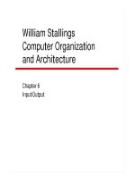
trade-offs and design decisions. Figure 15.2 illustrates this continuum from dedicated hardware
acceleration to software only.
Thus, we can look at performance in a slightly different light. We can also ask, “What are the
architectural trade-offs that must be made to achieve the desired performance objectives?
With the emergence of hardware description languages we can now develop hardware with the
same methodological focus on the algorithm that we apply to software. We can use object oriented
design methodology and UML-based tools to generate C++ or an HDL source file as the output
of the design. With this amount of fine-tuning available to the hardware component of the design
process, performance improvements can become incrementally achievable as the algorithm is
smoothly partitioned between the software component and the hardware component.
Overclocking
A very interesting subculture has developed around the idea of improving performance by over
-
clocking the processor, or memory, or both. Overclocking means that you deliberately run the

clock at a higher speed then it is supposedly designed to run at. Modern PC motherboards are
amazingly flexible in allowing a knowledgeable, or not-so-knowledgeable, user to tweak such
things as clock frequency, bus frequency, CPU core voltage and I/O voltage.
Search the Web and you’ll find many websites dedicated to this interesting bit of technology. Many
of the students whom I teach have asked me about it each year, so I thought that this chapter would
be an appropriate point to address it. Since overclocking is, by definition, violating the manufac
-
turer’s specifications, CPU manufacturers go out of their way to thwart the zealots, although the
results are often mixed.
Modern CPUs generally phase lock the internal clock frequency to the external bus frequency. A cir
-
cuit, called a phase-locked loop (PLL), generates an internal clock frequency that is a multiple of the
external clock frequency. If the external clock frequency is 200 MHz (PC3200 memory) and the mul
-
tiplier is 11, the internal clock frequency would be 2.2 GHz. The PLL circuit then divides the internal
clock frequency by 11 and uses the divided frequency to compare itself with the external frequency.
The local frequency difference is used to speed-up or slow down the internal clock frequency.
Figure 15.2: Hardware/software trade-off.
Slower Faster
Software
Hardware
Inexpensive Costly
Lower power consumption Increased power consumption
Programmable Inflexible
Performance Issues in Computer Architecture
403
You can overclock your processor by either:
1. Changing the internal multiplier of the CPU, or
2. Raising the external reference clock frequency.
CPU manufacturers deal with this issue by hard-wiring the multiplier to a fixed value, although

enterprising hobbyists have figured out how to break this code. Changing the external clock
frequency is relatively easy to do if the motherboard supports the feature, and may aftermarket
motherboard manufacturers have added features to cater to the overclocking community. In general,
when you change the external clock frequency you also change the frequency of the memory clock.
OK, so what’s the down side? Well, the easy answer is that the CPU is not designed to run faster
than it is specified to run at, so you are violating specifications when you run it faster than it is
designed to run. Let’s look at this a little deeper. An integrated circuit is designed to meet all of its
performance parameters over a specified range of temperature. For example the Athlon processor
from AMD is specified to meet its parametric specifications for temperatures less than 90 degrees
Celsius. Generally, every timing parameter is specified with three parameters, minimum, typical
and maximum (worst case) over the operating temperature range of the chip. Thus, if you took a
large number of chips and placed them on an expensive parametric testing machine, you would
discover a bell-shaped curve for most of the timing parameters of the chip. The peak of the curve
would be centered about the typical values and the maximum and minimum ranges define either
side of typical. Finally, the colder that you can maintain a chip, the faster it will go. Device physics
tells us that electronic transport properties in integrated circuits get slower as the chip gets hotter.
If you were to look closely at an IC wafer fully of just-processed Athlons or Pentiums, you would
also see a few different looking chips evenly distributed over the surface of the wafer. These chips
are the chips that are actually used to characterize the parameters of each wafer manufacturing batch.
Thus, if the manufacturing process happens to go really well, you get a batch of faster than typical
CPUs. If the process is marginally acceptable, you might get a batch of slower than typical chips.
Suppose that, as a manufacturer, you have really fine-tuned the manufacturing process to the point
that all of your chips are much better than average. What do you do? If you’ve ever purchased a
personal computer, or built one from parts, you know that faster computers cost more because the
CPU manufacturer charges more for the faster part. Thus, an Athlon XP processor that is rated at
3200+ is faster than an Athlon XP rated at 2800+ and should cost more. But suppose that all you
have been producing are the really fast ones. Since you still need to offer a spectrum of parts at
different price points, you mark the faster chips as slower ones.
Therefore, overclockers may use the following strategies:
1. Speed up the processor because it is likely to be either conservatively rated by the manu

-
facturer or is intentionally rated below its actual performance capabilities for marketing
and sales reasons,
2. Speed up the processor and also increase the cooling capability of your system to keep the
chip as cool as possible and to allow for the additional heat generated by a higher clock
frequency.
3. Raise either or both the CPU core voltage and the I/O voltage to decrease the rise and fall
times of the logic signals. This has the effect of raising the heat generated by the chip.
Chapter 15
404
4. Keep raising the clock frequency until the computer becomes unstable, then back off a
notch or two,
5. Raise the clock frequency, core voltage, I/O voltage until the chip self-destructs.
The dangers of overclocking should now be obvious:
1. A chip that runs hotter is more likely to fail,
2. Depending upon typical specs does not guarantee performance over all temperatures and
parametric conditions,
3. Defeating the manufacturers thresholds will void your warranty,
4. Your computer may be marginally stable and have a higher sensitivity to failures and
glitches.
That said should you overclock your computer to increase performance? Here’s a guideline to help
you answer that question:
If your PC is hobby activity, such as game box, then by all means, experiment with it. However, if
you depend upon your PC to do real work, then don’t tempt fate by overclocking it. If you really
want to improve your PC’s performance, add some more memory.
Measuring Performance
In the world of the
personal computer and the workstation, performance measurements are gen-
erally left to others. For example, most people are familiar with the
SPEC series of software

benchmark suites. The SPECint and SPECfp benchmarks measured integer and floating point
performance, respectively. SPEC is an acronym for the Standard Performance Evaluation Corpora
-
tion, a nonprofit consortium of computer manufacturers, system integrators, universities and other
research organizations. Their objective is to set, maintain and publish a set of relevant benchmarks
and benchmark results for computer systems
4
.
In response to the question, “Why use a benchmark?” The SPEC Frequently Asked Question page
notes,
Ideally, the best comparison test for systems would be your own application with your
own workload. Unfortunately, it is often very difficult to get a wide base of reliable,
repeatable and comparable measurements for comparisons of different systems on your
own application with your own workload. This might be due to time, money, confidential
-
ity, or other constraints.
The key here is that best benchmark test is your actual computing environment. However, few
people who are about to purchase a PC have the time or the inclination to load all of their software
on several machines and spend a few days with each machine, running their own software applica
-
tions in order to get a sense of relative strengths of each system. Therefore, we tend to let others,
usually the computer’s manufacturer, or a third-party reviewer, do the benchmarking for us. Even
then, it is almost impossible to be able to compare several machines on an absolutely even playing
field. Potential differences might include:
• Differences in the amount of memory in each machine,
• Differences in memory type in each machine, (PC2700 versus PC3200)
Performance Issues in Computer Architecture
405
• Different CPU clock rates,
• Different revisions of hardware drivers,

• Differences in the video cards,
• Differences in the hard disk drives (serial ATA or parallel ATA, SCSI or RAID)
In general, we will put more credence in benchmarks that are similar to the applications that we
are using, or intend to use. Thus, if you are interested in purchasing high-performance worksta
-
tions for an animation studio you likely choose from the graphics suite of tests offered by SPEC.
In the embedded world, performance measurements and benchmarks are much more difficult to
acquire and make sense of. The basic reason is that embedded systems are not standard platforms
the way workstations and PCs are standard. Almost every embedded system is unique in terms of
the CPU, clock speed, memory, support chips, programming language used, compiler used and
operating system used.
Since most embedded systems are extremely cost sensitive, there is usually little or no margin
available to design the system with more theoretical performance then it actually needs “just to
be on the safe side”. Also, embedded systems are typically used in real time control applications,
rather than computational applications. Performance of the system is heavily impacted by the
nature and frequency of the real time events that must be serviced within a well-defined window of
time or the entire system could exhibit catastrophic failure.
Imagine that you are designing the flight control system for a new fly-by-wire jet fighter plane.
The pilot does not control the plane in the classical sense. The pilot, through the control stick
and rudder pedals, sends requests to the flight control computer (or computers) and the computer
adjusts the wings and tail surfaces in response to the requests. What makes the plane so highly
maneuverable in flight also makes it difficult to fly. Without the constant control changes to the
flight surfaces, the aircraft will spin out of control. Thus, the computer must constantly monitor
the state of the aircraft and the flight control surfaces and make constant adjustments to keep the
fighter flying.
Unless the computer can read all of its input sensors and make all of the required corrections in the
appropriate time window, the aircraft will not be stable in flight. We call this condition
time criti-
cal. In other words, unless the system can respond within the allotted time, the system will fail.
Now, let’s change employers. This time you are designing some of the software for a color photo

printer. The Marketing Department has written a requirements document specifying a 4 page-per-
minute output delivery rate. The first prototypes actually deliver 3.5 pages per minute. The printer
keeps working, no one is injured, but it still fails to meet its design specifications. This is an example
of a time sensitive application. The system works, but not as desired. Most embedded applications
with real-time performance requirements fall into one or the other of these two categories.
The question still remains to be answered, “What benchmarks are relevant for embedded sys
-
tems?” We could use the SPEC benchmark suites, but are they relevant to the application domain
that we are concerned with. In other words, “How significant would a benchmark that does a prime
number calculation be in comparing the potential use of one of three embedded processors in a
furnace control system?”
Chapter 15
406
For a very long time there were no benchmarks suitable for use by the embedded systems com-
munity. The available benchmarks were more marketing and sales devices then they were usable
technical evaluation tools. The most notorious among them was the MIPS benchmark. The
MIPS
benchmark means millions of instructions per second. However, it came to mean,
Meaningless Indicator of Performance for Salesmen.
The MIPs benchmark is actually a relative measurement comparing the performance of your CPU
to a VAX 11/780 computer. The 11/780 is a 1 MIPS machine that can execute 1757 loops of the
Dhrystone
5
benchmark in 1 second. Thus, if your computer executes 2400 loops of the benchmark,
it is a 2400/1757 = 1.36 MIPS machine. The Dhrystone benchmark is a small C, Pascal or Java
program which compiles to approximately 2000 lines of assembly code. It is designed to test the
integer performance of the processor and does not use any operating system services.
There is nothing inherently wrong with the Dhrystone benchmark, except that people started using
it to make technical decisions which created economic impacts. For example, if we choose pro
-

cessor A over processor B because its better Dhrystone benchmark results, that could result in the
customer using many thousands of A-type processors in their new design. How could you make
your processor look really good in a Dhrystone benchmark? Since the benchmark is written in a
high-level language, a compiler manufacturer could create specific optimizations for the Dhrystone
benchmark. Of course, compiler vendors would never do something like that, but everyone con
-
stantly accused each other of similar shortcuts. According to Mann and Cobb
6
,
Unfortunately, all too frequently benchmark programs used for processor evaluation are
relatively small and can have high instruction cache hit ratios. Programs such as Dhrys
-
tone have this characteristic. They also do not exhibit the large data movement activities
typical of many real applications.
Mann and Cobb cite the following example,
Suppose you run Dhrystone on a processor and find that the µP (microprocessor) executes
some number of iterations in P cycles with a cache hit ratio of nearly 100%. Now, suppose
you lift a code sequence of similar length from your application firmware and run this
code on the same µP. You would probably expect a similar execution time for this code.
To your dismay, you find that the cache hit rate becomes only 80%. In the target system,
each cache miss costs a penalty of 11 processor cycles while the system waits for the
cache line to refill from slow memory; 11 cycles for a 50 MHz CPU is only 220 ns. Execu
-
tion time increases from P cycles for Dhrystone to (0.8 x P) + (0.2 x P x 11) = 3P. In other
words, dropping the cache hit rate to 80% cuts overall performance to just 33% of the
level you expected if you had based your projection purely on the Dhrystone result.
In order to address the benchmarking needs of the embedded systems industry, a consortium or
chip vendors and tool suppliers was formed in 1997 under the leadership of Marcus Levy, who
was a Technical Editor at EDN magazine. The group sought to create,
meaningful performance

benchmarks for the hardware and software used in embedded systems
7
. The EDN Embedded
Microprocessor Benchmark Consortium (EEMBC, pronounced “Embassy”) uses real-world
benchmarks from various industry sectors.
Performance Issues in Computer Architecture
407
The sectors represented are:
• Automotive/Industrial
• Consumer
• Java
• Networking
• Office Automation
• Telecommunications
• 8 and 16-bit microcontrollers
For example, in the Telecommunications group there are five categories of tests; and within each
category there are several different tests. The categories are:
• Autocorrelation
• Convolution encoder
• Fixed-point bit allocation
• Fixed-point complex FFT
• Viterbi GSM decoder
If these seem a bit arcane to you, they most
certainly are. These are algorithms that are
deeply ingrained into the technology of the
Telecommunications industry. Let’s look at
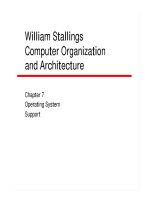
an example result for the EEMBC Autocor
-
relation benchmark on a 750 MHz Texas
Instruments TMS320C4X Digital Signal

Processor (DSP) chip. The results are shown
in Figure 15.3.
The bar chart shows the benchmark using a
C compiler without optimizations turned on;
with aggressive optimization; and with hand-
crafted assembly language fine-tuning. The results are pretty impressive. There is a almost a 100%
improvement in the benchmark results when the already optimized C code is further refined by
hand crafting in assembly language. Also, both the optimized and assembly language benchmarks
outperformed the nonoptimized version by factors of 19.5 and 32.2, respectively.
Let’s put this in perspective. All other things being equal, we would need to increase the clock
speed of the out-of-the-box result from 750 MHz to 24 GHz to equal the performance of the hand-
tuned assembly language program benchmark.
Even though the EEMBC benchmark is vast improvement there are still factors that can render
comparative results rather meaningless. For example, we just saw the effect of the compiler opti
-
mization on the benchmark result. Unless comparable compilers and optimizations are applied to
the benchmarks, the results could be heavily skewed and erroneously interpreted.
Another problem that is rather unique to embedded systems is the issue of hot boards. Manufac-
turers build evaluation boards
with their processors on them so that embedded system designers
Figure 15.3: EEMBC benchmark results for the
Telecommunications group Autocorrelation
benchmark
8
.
700
600
500
400
300

200
100
out of
the box
C optimized
Assembly
Optimized
19.5
379.1
628
EEMBC Autocorrelation benchmark
for the TMS320C64X
Chapter 15
408
who don’t yet have hardware available can execute
benchmark code or other evaluation programs on
the processor of interest. The evaluation board is
often priced above what a hobbyist would be will
-
ing to spend, but below what a first-level manager
can directly approve. Obviously, as a manufacturer, I
want my processor to look its best during a potential
design win test with my evaluation board. Therefore,
I will maximize the performance characteristics of
the evaluation board so that the benchmarks come out
looking as good as possible. Such boards are called
hot boards and they usually don’t represent the per
-
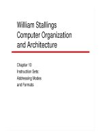
formance characteristics of the real hardware. Figure
15.4 is an evaluation board for the AMD AM186EM

microcontroller. Not surprising, it was priced at $186.
The evaluation board contained the fastest version
of the processor then available (40 MHz), and RAM
memory that is fast enough to keep up without any
additional wait states. All that is necessary to begin
to use the board is to add a 5 volt DC power supply and an RS232 cable to the COM port on your
PC. The board comes with an on-board monitor program in ROM that initiates a communications
session on power-up. All very convenient, but you must be sure that this reflects the actual operat
-
ing conditions of your target hardware.
Another significant factor to consider is whether or not your application will be running under an
operating system. An operating system introduces additional overhead and can decrease perfor
-
mance. Also, if your application is a low-priority task, it may become starved for CPU cycles as
higher priority tasks keep interrupting.
Generally, all benchmarks are measured relative to a timeline. Either we measure the amount of
time it takes for a benchmark to run, or we measure the number of iterations of the benchmark
that can run in a unit of time, day a second or a minute. Sometimes we can easily time events that
take enough time to execute that we can use a stopwatch to measure the time between writes to
the console. You can easily do this by inserting a
printf() or cout statement in your code. But what
if the event that you’re trying to time takes milliseconds or microseconds to execute? If you have
operating system services available to you then you could use a high resolution timer to record
your entry and exit points. However, every call to an O/S service or to a library routine is a poten
-
tially large perturbation on the system that you are trying to measure; a sort of computer science
analog of Heisenberg’s Uncertainty Principle.
In some instances, evaluation boards may contain I/O ports that you could toggle on and off. With
an oscilloscope, or some other high-speed data recorder you could directly time the event or events
with minimal perturbation on the system. Figure 15.5 shows a software timing measurement made

using an oscilloscope to record the entry and exit points to a function. Referring to the figure,
Figure 15.4: Evaluation board for the
AM186EM-40 Microcontroller from AMD.
Performance Issues in Computer Architecture
409
when the function is entered an I/O pin is turned
on and then off, creating a short pulse. On exit,
the pulse is recreated. The time difference be
-
tween the two pulses measures the amount of time
taken by the function to execute. The two verti
-
cal dotted lines are cursors that can be placed on
the waveform to determine the timing reference
marks. In this case, the time difference between
the two cursors is 3.640 milliseconds.
Another method is to use the digital hardware
designer’s tool of choice, the logic analyzer.
Figure 15.6 is photograph of a TLA7151 logic
analyzer manufactured by Tektronix, Inc. In
the photograph the logic analyzer has a multi-
wire connected to the busses of the computer
board through a dedicated cable. It is a common
practice, and a good idea, for the circuit board
designer to provide a dedicated port on the board to
enable a logic analyzer to easily be connected to the
board. The logic analyzer allows the designer to record
the state of many digital bits at the same time. Imagine
that you could simultaneously record and timestamp
1 million samples of a digital system that is 80 digital

bits wide. You might use 32 bits for the data, 32-bits
for the address bus, and the remaining 16-bits for vari
-
ous status signals. Also, the circuitry within the logic
analyzer can be programmed to only record a specific
pattern of bits. For example, suppose that we pro
-
grammed the logic analyzer to record only data writes
to memory address 0xAABB0000. The logic analyzer
would monitor all of the bits, but only record the
32-bits on the data bus whenever the address matches
0xAABB00 AND the status bits indicate a data write
is in process. Also, every time that the logic analyzer
records a data write event, it time stamps the event and records the time along with the data.
The last element of this example is for us to insert the appropriate reference elements into our code
so that the logic analyzer can detect them and record when they occur. For example, let’s say that
we’ll use the bit pattern 0xAAAAXXXX for the entry point to a function and 0x5555XXXX for
the exit point. The ‘X’s’ mean “don’t care” and may be any value, however, we would probably
want to use them to assign unique identifiers to each of the functions in the program.
Let’s look at a typical function in the program. Here’s the function:
Figure 15.5: Software performance Measure-
ment made using an oscilloscope to measure
the time difference between a function entry
and exit point.
Figure 15.6: Photograph of the Tektronix
TLA7151 logic analyzer. The cables from
the logic analyzer probe the bus signals of
the computer board. Photograph courtesy
of Tektronix, Inc.
Chapter 15

410
int typFunct( int aVar, int bVar, int cVar)
{
/* Lines of code */



}
Now, let’s add our measurement “tags.” We call this process instrumenting the code. Here’s the
function with the instrumentation added:
int typFunct( int aVar, int bVar, int cVar)
{
*(volatile unsigned int*) 0xAABB0000 = 0xAAAA03E7
/* Lines of code */



*(volatile unsigned int*) 0xAABB0000 = 0x555503E7
}
This rather obscure C statement,
*(unsigned int*) 0xAABB0000 =
0xAAAA03E7 creates a pointer to the
address 0xAABB0000 and immediately
writes the value 0xAAAA03E7 to that
memory location. We can assume that
0x03E7 is the code we’ve assigned to
the function, typFunct(). This statement
is our tag generator. It creates the data
write action that the logic analyzer can
then capture and record. The keyword,

volatile, tells the compiler that this write
should not be cached. The process is
shown schematically in Figure 15.7.
Let’s summarize the data shown in
Figure 15.7 in a table.
Figure 15.7 Software performance measurement made
using a logic analyzer to record the function entry and
exit point.
Host computer
System under test
Memory
CPU
Logic analyzer
Address bus
Data bus
Status bus
Partial Trace Listing
Address Data Time(ms)
AABB0000 AAAA03E7 145.87503
AABB0000 555503E7 151.00048
AABB0000 AAAA045A 151.06632
AABB0000 5555045A 151.34451
AABB0000 AAAAC40F 151.90018
AABB0000 5555C40F 155.63294
AABB0000 AAAA00A4 155.66001
AABB0000 555500A4 157.90087
AABB0000 AAAA2B33 158.00114
AABB0000 55552B33 160.62229
AABB0000 AAAA045A 160.70003
AABB0000 5555045A 169.03414

Function Entry/Exit(msec) Time difference
03E7 145.87503 / 151.00048 5.12545
045A 151.06632 / 151.34451 0.27819
C40F 151.90018 / 155.63294 3.73276
00A4 155.66001 / 157.90087 2.24086
2B33 158.00114 / 160.62229 2.62115
045A 160.70003 / 169.03414 8.33411
Performance Issues in Computer Architecture
411
Referring to the table, notice how the function labeled 045A has two different execution times,
0.27819 and 8.33411, respectively. This may seem strange but it actually quite common. For
example, a recursive function may have different execution times as well as functions which call
math library routines. However, it might also indicate that the function is being interrupted and
that the time window for this function may vary dramatically depending upon the current state of
the system and I/O activity.
The key here is that the measurement is almost as unobtrusive as you can get. The overhead of a
single write to noncached memory should not distort the measurement too severely. Also, notice
the logic analyzer is connected to another host computer. Presumably this host computer was the
one that was used to do the initial source code instrumentation. Thus, it should have access to the
symbol table and link map. Therefore, it could present the results by actually providing the func
-
tion’s names rather than a identifier code.
Thus, if were to run the system under test for a long enough span of time we could continue to
gather data like that shown in Figure 15.7 and then do some simple statistical analyses to deter
-
mine min, max and average execution times for the functions.
What other types of performance data would this type of measurement allow us to obtain? Some
measurements are summarized below:
1. Real-time trace: Recording the function entry and exit points provides a history of the execu
-

tion path taken by the program as it runs in real-time. Rather than single-stepping, or running
to a breakpoint, this debugging technique does not stop the execution flow of the program.
2. Coverage testing: This test keeps track of the portions of the program that were executed
and portions that were not executed. This is valuable for locating regions of dead code and
additional validation tests that should be performed.
3. Memory leaks: Placing tags at every place where memory is dynamically allocated and
deallocated can determine if the system has a memory leakage or fragmentation problem.
4. Branch analysis: By instrumenting program branches these tests can determine if there are
any paths through the code that are not traceable or have not been thoroughly tested. This
test is one of the required tests for any code that is deemed to be
mission critical and must
be certified by a government regulatory agency before it can be deployed in a real product.
While a logic analyzer provides a very low-intrusion testing environment, all computer systems
can’t be measured in this way. As previously discussed, if an operating system is available, then
the tag generation process and recording can be accomplished as another O/S task. Of course, this
is obviously more intrusive, but may be a reasonable solution for certain situations.
At this point, you might be tempted to suggest, “Why bother with the tags? If the logic analyzer
can record everything happening on the system busses, why not just record everything?” This is
a good point and it would work just fine for noncached processors. However, as soon as you have
a processor with on-chip caches, bus activity ceases to be a good indicator of processor activity.
That’s why tags work so well.
While logic analyzers work quite well for these kinds of measurements, they do have a limitation
because they must stop collecting data and upload the contents of their trace memory in batches.
Chapter 15
412
This means that low duty cycle events, such as
interrupt service routines, may not be captured.
There are commercially available products, such
as CodeTest® from Metrowerks®
9

that solves
this problem by able to continuously collect tags,
compress them, and send them to the host without
stopping. Figure 15.8 is a picture of the CodeTest
system and Figure 15.9 shows the data from a
performance measurement.
Designing for Performance
One of the most important reasons that a
software student should study computer ar
-
chitecture is to understand the strengths and
limitations of the machine and the environ
-
ment that their software will be running in.
Without a reasonable insight into the opera
-
tional characteristics of the machine, it would
be very easy to write inefficient code. Worse
yet, it would be very easy to mistake inef
-
ficient code for limitations in the hardware
platform itself. This could lead to a decision
to redesign the hardware in order to increase
the system performance to the desired level,
even though a simple re-write of some criti-
cal functions may be all that is necessary.
Here’s a story of an actual incident that illustrates this point:
A long time ago in a career far, far away I was the R&D Director for the CodeTest prod
-
uct line. A major Telecomm manufacturer was considering making a major purchase of

CodeTest equipment so we sent a team from the factory to demonstrate the product. The
customer was about to go into a redesign of a major Telecomm switching system that they
sold because they thought that they had reached the limit of the hardware’s performance.
Our team visited their site and we installed a CodeTest unit in their hardware. After run
-
ning their switch for several hours we all examined the data together. Of the hundreds
of functions that we looked at, none of the engineers could identify the one function that
was using 15% of the CPU’s time. After digging through the source code the engineers
discovered a debug routine that was added by a student intern. The intern was debugging
a portion of the system as his summer project. In order to trace program flow, he created
a high priority function that flashed a light on one of the switch’s circuit boards. Being an
intern, he never bothered to properly identify this function as a temporary debug function
and it somehow it got wrapped into the released product code.
Figure 15.8: CodeTest software performance
analyzer for real-time systems. Courtesy of
Metrowerks, Inc.
Figure 15.9: CodeTest screen shot showing a software
performance measurement. The data is continuously
updated while the target system runs in real-time.
Courtesy of Metrowerks, Inc.
Performance Issues in Computer Architecture
413
After removing the function and rebuilding the files, the customer gained an additional
15% of performance headroom. They were so thrilled with the results that they thanked us
profusely and treated us to a nice dinner. Unfortunately, they no longer needed the Co
-
deTest instrument and we lost the sale. The moral of this story is that no one bothered to
really examine the performance characteristics of the system. Everyone assumed that their
code ran fine and the system as whole performed optimally.
Stewart

10
notes that the number one mistake made by real-time software developers is not know-
ing the actual execution time of their code. This is not just an academic issue, even if the software
that is being developed is for a PC or workstation, getting the most performance from your system
is like any other form of engineering. You should endeavor to make the most efficient use of the
resources that you have available to you.
Performance issues are most critical in systems that have limited resources, or have real-time per
-
formance constraints. In general, this is the realm of most embedded systems so we’ll concentrate
our focus in this arena.
Ganssle
11
argues that you should never write an interrupt service routine in C or C++ because the
execution time will not be predictable. The only way to approach predictable code execution is by
writing in assembly language. Or is it? If you are using a processor with an on chip cache, how do
you know what the cache hit ratio will be for your code? The ISR could actually take significantly
longer to run than the assembly language cycle count might predict.
Hillary and Berger
12
describe a 4-step process to meet the performance goals of a software design
effort:
1. Establish a performance budget,
2. Model the system and allocate the budget,
3. Test system modules,
4. Verify the performance of the final design.
The performance budget can be defined as:
Performance budget = sum(operations require under worst case conditions)
= [1/ (data rate)] – Operating system overhead – headroom
The data rate is simply the rate that data is being generated and will need to be processed. From
that, you must subtract the overhead of the operating system and finally, leave some room for the

code that will invariably need to add as additional features get added-on.
Modeling the system means decomposing the budget into functional blocks that will be required
and allocating time for each block. Most engineers don’t have a clue about amount of time
required for different functions, so they make “guesstimates”. Actually, this isn’t so bad because
at least they are creating a budget. There are lots of ways to refine these guesses without actually
writing the finished code and testing it after the fact. The key is to raise an awareness level of the
time available versus time needed.
Once software development begins it makes sense to test the execution time at the module
level, rather than wait for the integration phase to see if your software’s performance meets the
Chapter 15
414
requirements specifications. This will give you instant feedback about how the code is doing
against budget. Remember, guesses can go either way, too long or too short, so you might have
more time than you think (although Murphy’s Law will usually guarantee that this is a very low
probability event).
The last step is to verify the final design. This means performing accurate measurements of the
system performance using some of the methods that we’ve already discussed. Having this data will
enable you to sign off on the software requirements documents and also provide you with valuable
data for later projects.
Best Practices
Let’s conclude this chapter with some best practices. There are hundreds of them, far too many for
us to cover here. However, let’s get a flavor for some performance issues and some do’s and don’ts.
1. Develop a requirements document and specifications before you start to write code. Fol
-
low an accepted software development process. Contrary to what most students think,
code hacking is not an admired trait in a professional programmer. If possible, involve
yourself in the system’s architectural design decision before they are finalized. If there is
no other reason to study computer architecture, this is the one. Bad partitioning decisions
at the beginning of project usually lead to pressure on the software team to fix the mess at
the back end of the project.

2. Use good programming practices. The same rules of software design apply whether you
are coding for a PC or for an embedded controller. Have a good understanding of the gen
-
eral principles of algorithm design. For example, don’t use O(n
2
) algorithms if you have a
large dataset. No matter how good the hardware, inefficient algorithms can stop the fastest
processor.
3. Study the compiler that you’ll be using and understand how to take fullest advantage of
it. Most industrial quality compilers are extremely complicated programs and are usually
not documented in a way that mere mortals could comprehend. So, most engineers keep
on using the compiler in the way that they’ve used it in the past, without regard for what
kind of incremental performance benefits they might gain by exploring some of the avail
-
able optimization options. This is especially true if the compiler itself is architected for a
particular CPU architecture. For example, there was a version of the GNU®
12
compiler for
the Intel i960 processor family that could generate performance profile data from an ex
-
ecuting program and then use that data on subsequent compile-execute cycles to improve
the performance of the code.
4. Understand the execution limits of your code. For example, Ganssle
14
recommends that in
order to decide how much memory to allocate for the stack, you should fill the stack region
with an identifiable memory pattern, such as 0xAAAA or 0x5555. Then run your program
for enough time to convince yourself that it has been thoroughly exercised. Now, look at
the high water mark for the stack region by seeing where your bit pattern was overwritten.
Then add a safety factor and that is your stack space. Of course, this implies that your code

will be deterministic with respect to the stack. One of the biggest don’ts in high-reliability
software design is to use recursive functions. Each time a recursive function calls itself,
Performance Issues in Computer Architecture
415
it creates a stack frame that continues to build the stack. Unless you absolutely know
the worst-case recursive function call sequence, don’t use them. Recursive functions are
elegant, but they are also dangerous in systems with strictly defined resources. Also, they
have a significant overhead in the function call and return code, so performance suffers.
5. Use assembly language when absolute control is needed. You know how to program in as
-
sembly language, so don’t be afraid to go in and do some handcrafting. All compilers have
mechanisms for including assembly code in your C or C++ programs. Use the language
that meets the required performance objectives.
6. Be very careful of dynamic memory allocation when you are designing for any embedded
system, or other system with a high-reliability requirement. Even without a designed in
memory leak, such as forgetting to free allocated memory, or a bad pointer bug, memory
can become fragmented if the memory handler code is not well-matched to your applica-
tion.
7. Do not ignore all of the exception vectors offered by your processor. Error handlers are
important pieces of code that help to keep your system alive. If you don’t take advantage
of them, or just use them to vector to a general system reset, you’ll never be able to track
down why the system crashes once every four years on February 29
th
.
8. Make certain that you and the hardware designers agree on which Endian model you are
using.
9. Be judicious in your use of global variables. At the risk of incurring the wrath of Com
-
puter Scientists I won’t say, “Don’t use global variables” because global variables provide
a very efficient mechanism for passing parameters. However, be aware that there are

dangerous side effects associated with using globals. For example, Simon
15
illustrates the
problem associated with memory buffers, such as global variables in his discussion of the
shared-data problem. If a global variable is used to hold shared data then a bug could be
introduced if one task attempts to read the data while another task is simultaneously writ-
ing it. System architecture can affect this situation because the size of the global variable
and the size of the external memory could create a problem in one system and not be a
problem in another system. For example, suppose a 32-bit value is being used as a global
variable. If the memory is 32-bits wide, then it takes one memory write to change the
value of the variable. Two tasks can access the variable without a problem. However, if the
memory is 16 bits wide, then two successive data writes are required to update the vari-
able. If the second task interrupts the first task after the first memory access but before the
second access, it will read corrupted data.
10. Use the right tools to do the job. Most software developers would attempt to debug a
program without a good debugger. Don’t be afraid to use an oscilloscope or logic analyzer
just because they are “Hardware Designer’s Tools.”
Chapter 15
416
Summary of Chapter 15
Chapter 15 covered:
• How various hardware and software factors will impact the actual performance of a
computer system.
• How performance is measured.
• Why performance does not always mean “as fast as possible.”
• Methods used to meet performance requirements.
Chapter 15: Endnotes
1
Linley Gwennap, A numbers game at AMD, Electronic Engineering Times, October 15, 2001.
2

(Justin Rattner is an Intel Fellow at Intel Labs.).
3
Arnold S. Berger, Embedded System Design, ISBN 1-57820-073-3, CMP Books, Lawrence, KS, 2002, p. 9.
4
/>5
R.P. Weicker, Dhrystone: A Synthetic Systems Programming Benchmark, Communications of the ACM, Vol. 27,
No. 10, October, 1984, pp. 1013–1030.
6
Daniel Mann and Paul Cobb, Why Dhrystone Leaves You High and Dry, EDN, May 1998.
7
/>8
Jackie Brenner and Markus Levy, Code Efficiency and Compiler Directed Feedback, Dr. Dobb’s Journal, #355,
December 2003, p. 59.
9
www.metrowerks.com.
10
Dave Stewart, The Twenty-five Most Common Mistakes with Real-Time Software Development,” a paper presented at
the Embedded Systems Conference, San Jose, CA, September 2000.
11
Jack Ganssle, The Art of Designing Embedded Systems, ISBN 0-7506-9869-1, Newnes, Newnes, Boston, MA, p. 91.
12
Nat Hillary and Arnold Berger, Guaranteeing the Performance of Real-Time Systems, Real Time Computing, October,
2001, p. 79.
13
www.gnu.org.
14
Jack Ganssle, op cit, p. 61.
15
David E. Simon, An Embedded Software Primer, ISBN 0-201-61569-X, Addison-Wesley, Reading, MA, 1999, p. 97.
417

1. People who enjoy playing video games on their PC’s will often add impressive liquid cooling
systems to remove heat from the CPU. Why?
2. Why will adding more memory to your PC often have more of an impact on performance then
replacing the current CPU with a faster one?
3. Assume that you are trying to compare the relative performance of two computers. Computer
#1 has a clock frequency of 100 MHz. Computer #2 has a clock frequency of 250 MHz.
Computer #1 executes all of its instructions in its instruction set in 1 clock cycle. On average,
computer #2 executes 40% of its instruction set in one clock cycle and the rest of its instruc
-
tion set in two clock cycles. How long will it take each computer to run a benchmark program
consisting of 1000 instructions in a row, followed by a loop of 100 instructions that executes
200 times.
Note: You may assume that for computer #2 the instructions in the benchmark are randomly distributed in a way
that matches the overall performance of the computer as stated above.
4. Discuss three ways that, for a given instruction set architecture, processor performance may be
improved.
5. Suppose that, on average, computer #1 requires 2.0 cycles per instruction, and uses a 1GHz
clock frequency. Computer #2 averages 1.2 cycles per instruction and has a 500 MHz clock.
Which computer has the better relative performance? Express your answer as a percentage.
6. Suppose that you are trying to evaluate two different compilers. In order to do this you take
one of the standard benchmarks and separately compile it to assembly language using each
compiler. The instruction set architecture of this particular processor is such that the assembly
language instructions may be grouped into 4 categories according to the number of CPU clock
cycles required to execute each instruction in the category. This is shown in the table below:
Exercises for Chapter 15
Instruction category CPU cycles required to execute
Category A 2
Category B 3
Category C
4

Category D 6
You look at the assembly language output of each of the compilers and determine the relative
distribution of each instruction category produced by the compiler.
Chapter 15
418
Compiler A compiled the program to 1000 assembly language instructions and produced the
distribution of instructions shown below:
Instruction category % of instructions in each category
Category A 40
Category B 10
Category C 30
Category D 20
Compiler B compiled the program to 1200 assembly language instructions and produced the
distribution of instructions shown below:
Instruction category % of instructions in each category
Category A 60
Category B 20
Category C 10
Category D 10
Which compiler would you expect to give better performance with this benchmark program?
Why? Be as specific as possible.
7. Suppose that you are considering the design trade-offs for an extremely cost-sensitive product.
In order to reduce the hardware cost you consider using a version of the processor with an
8-bit wide external data bus instead of the version with the 16-bit wide data bus. Both versions
of the processor run at the same clock frequency and are fully 32-bits wide internally. What
type of performance difference would you expect to see if you were trying to sum 2, 32-bit
wide memory variables with the sum also stored in memory.
8. Why would a compiler try to optimize a program by maximizing the size and number of basic
blocks in the code? Recall that a basic block is a section of code with one entry point, one exit
point and no internal loops.

419
C H A P T E R
16
Future Trends and
Reconfigurable Hardware
Objectives
When you are finished this lesson, you will be able to describe:
 How programmable logic is implemented;
 The basic elements of the ABEL programming language;
 What is reconfigurable hardware and how it is implemented;
 The basic architecture of a field programmable gate array;
 The architecture of reconfigurable computing machines;
 Some future trends in molecular computing;
 Future trends in clockless computing.
Introduction
We’ve come a long way since Chapter 1, and this chapter is a convenient place to stop and take
a forward look to where all of this seems to be going. That is not to say that we’ll make a leap to
the Starship Enterprise’s on-board computer (although that would be a fun thing to do), but rather,
let’s look a where the trends that are in place today seem to be leading us. Along the way, we’ll
look at a topic that is emerging in importance but we’ve just not had a convenient place to discuss
it until now.
The focus of this text has been to view the hardware as it is relevant to a software developer. One
of the trends that has been going on for several years and continues to grow is the blurring of the
lines between what is hardware and what is software. Clearly, software is the driving code for the
hardware state machine. But what if the hardware itself was programmable, just like a software
algorithm? Can you imagine a computing engine that had no personality at all until the software is
loaded? In other words, the distinction between 68K, x86 or ARM would not exist at all until you
load a new program. Part of the program actually configures the hardware to the desired architec
-
ture. Science fiction you say? Not all. Read on.

Reconfigurable Hardware
From a historical perspective, configurable hardware arrived in the 1970’s with the arrival of a digi-
tal integrated circuit called a PAL, or programmable array logic. A PAL was designed to contain a
collection of general purpose gates and flip-flops, organized in a manner that would allow a design
-
er to easily create simple to moderately complex sum-of-products logic circuits or state machines.
Chapter 16
420
The gate shown in Figure 16.1 is a non-
inverting buffer gate. A gate that doesn’t
provide a logic function may seem strange,
but sometimes the purity of logic must
yield to the realities of the electronic
properties of digital circuits and we need a
circuit with noninverting logic from input
to output. What is of interest to us in this
particular example is the configuration of
the output circuitry of the gate. This type
of circuit configuration is called either
open collector or open drain, depending
upon the type of integrated circuit technol
-
ogy that is being used. For our purposes,
open collector is the more generic term, so
we’ll use it exclusively.
An open-collector output is very similar to a tri-state output, but with some differences. Recall that
a tri-state output is able to isolate the logic function of the device (1 or 0) from the output pin of
the device. An open collector device works in a similar manner, but its purpose is not to isolate the
input logic from the output pin. Rather, the purpose is to enable multiple outputs to be tied together
in order to implement logic functions such as AND and OR. When we implement an AND func

-
tion by tying together the open collector gate outputs we call the circuit a wired-AND output.
In order to understand how the circuit works
imagine that you are looking into the output
pin of the gate in Figure 16.1. If the gate
input is at logic zero, then you would see
that the open collector output “switch” is
closed, connecting the output to ground,
or logic level 0. If the input is 1, the output
switch is opened, so there is no connec-
tion to anything. The switch is in the high
impedance state, just like a tri-state gate.
Thus, the open collector gate has two states
for the output, 0 or high impedance.
Figure 16.2 illustrates a 3-input wired AND
function. For the moment please ignore
the circuit elements labeled F1, F2 and F3.
These are fuses that can be permanently
“blown”. We’ll discuss their purpose in
a moment. Since all three gates are open
collector devices, either their outputs are
Figure 16.1: Simplified schematic diagram of a non-
inverting buffer gate with an open collector output
configuration.
OC
OC
Switch
open
1
Switch

close
d
0
OUT
IN
Figure 16.2: 3-input wired AND logic function. The
circuit symbols labeled F1, F2 and F3 are fuses
which may be intentionally destroyed, leaving the
gate output permanently removed from the logic
equation.
A
B
C
3.3V
Y = A * B * C
F1
F2
F3
Resistor
Future Trends and Refigurable Hardware
421
connected to ground (logic 0) or in the Hi-Z state. If all three inputs A, B and C are logic 1, then
all three outputs are Hi-Z. This means that none of the outputs are connected to the common wire.
However, the resistor ties the wire to the system power supply, so you would see the wire as a
logic level 1. The difference is that the logic 1 is being supplied by the power supply through the
resistor, rather than the output of a gate. We refer to the resistor as a pull-up resistor
because it is
pulling the voltage on the wire “up” to the voltage of the power supply.
If input A, B or C is at logic 0, then the wire is connected to ground. The resistor is needed to pre
-

vent the power supply from being directly connected to ground, causing a short circuit, with lots of
interesting circuit pyrotechnics and interesting odors. The key is that the resistor limits the current
that can flow from the power supply to ground to a safe value and also provides us with a reference
point to measure the logic level. Also, it doesn’t matter how many of the gates inputs are at logic 0,
the effect is still to connect the entire wire to ground, thus forcing the output to a logic 0.
The fuses, F1, F2 and F3 add another dimension to the circuit. If there was a way to vaporize the
wire that makes up the fuse, say with a large current pulse, then that particular open collector gate
would be entirely removed from the circuit. If we blow fuse F3, then the circuit is a 2-input and
gate, consisting of inputs A and B and output Y. Of course, once we decide to blow a fuse we can’t
put it back the way it was. We call such a device one-time programmable
, or an OTP device.
Figure 16.3 shows how we can extend
the concept of the wired AND function
to create a general purpose device that
is able to implement an arbitrary sum
of products logic function in four inputs
and two outputs within a single device.
The circles in the figure represent pro
-
grammable cross-point switches. Each
switch could be an OTP fuse, as in Fig
-
ure 16.2, or an electronic switch, such as
the output switch of a tri-state gate. With
electronic switches we would also need
some kind of additional configuration
memory to store the state of each cross-
point switch, or some other means to reprogram the switch when desired. Notice how each input is
converted to the input and its complement by the input/invert box. Each of the inputs and comple
-

ments then connect to each of the horizontal wires in the array. The horizontal wires implement the
wired “AND’ function for the set of the vertical wires. By selectively programming the cross-point
switches of the AND plane, each OR gate output can be any single level sum of products term.
Figure 16.4 shows the pin outline diagram for two industry standard PAL devices, the 16R4 and
16L8. Referring to the 16L8 we see that the part has 10 dedicated inputs (pins 1 through 9 and pin
11), 6 pins that may be configured to be either inputs or outputs (pins 12 through 18), and two pins
that are strictly for outputs (12 and 19). The other device in Figure 16.4, the 16R4 is similar to the
16L8 but it includes 4 ‘D’ type flip-flop devices that facilitate the design of simple state machines.
Figure 16.3: Simplified schematic diagram of a portion of
a programmable array logic, or PAL device.
A B C D
A A B B C C D D
X
Y
OR
OR
=
Programmable
Interconnect
Input/Invert
“Wired”
AND
plane
a
b
c
d
e
f
g

h
Chapter 16
422
Even with relatively simple devices
such as these, the number of inter-
connection points which must be
programmed quickly numbers in
the hundreds or thousands. In order
to bring the complexity under con
-
trol, the Data I/O Corporation®
1
, a
manufacturer of programming tools
for programmable devices, invented
one of the earliest hardware descrip
-
tion languages, called ABEL, which
is an acronym for
Advanced Boolean
Equation Language. Today ABEL is an
industry-standard hardware description
language. The rights to ABEL are now
owned by the Xilinx Corporation, a San Jose, California-based manufacturer of programmable
hardware devices and programming tools.
ABEL is a simpler language than Verilog or VHDL, however it is still capable of defining fairly
complex circuit configurations. Here’s a partial example of an ABEL source file. The process is as
follows:
1. Create an ASCII based source file, source.abl
2. Compiler the source file to create a programming map called source.jed

.
3. The source.jed file is downloaded to a device programmer, such as the type built by
Data I/O, and the device is programmed by “blowing” (removing) the appropriate
fuses for a OTP part, or turning on the appropriate cross-point switches if the device is
reprogrammable.
Some of the appropriate declarations are shown below. The keywords are shown in bold.
module AND-OR;
title
Designer Arnold Berger
Revision 2
Company University of Washington-Bothell
Part Number U52
declarations
Figure 16.4: Pin-out diagrams for the industry standard
16L8 and 16R4 PALs.
1
2
3
4
5
6
7
8
9
10
20
19
18
17
16

15
14
13
12
11
CP
I
I
I
I
I
I
I
I
GND
V
CC
I/O
I/O
O
O
O
O
I/O
I/O
OE
AND
OR
GATE
ARRAY

16R4
1
2
3
4
5
6
7
8
9
10
20
19
18
17
16
15
14
13
12
11
I
I
I
I
I
I
I
I
I

GND
V
O
I/O
I/O
I/O
I/O
I/O
I/O
O
I
AND
OR
GATE
ARRA
Y
16L8
Future Trends and Refigurable Hardware
423
“ Inputs
AND-OR Device PAL20V10 ;
a1 pin 1 ;
b1 pin 2 ;
b2 pin 3 ;
b3 pin 4 ;
b4 pin 5 ;
c1 pin 6 ;
c2 pin 7 ;
c3 pin 8 ;
c4 pin 9 ;

a4 pin 19 ;
a3 pin 18 ;
a2 pin 17 ;
“Outputs
zc pin 11 istype ‘com,buffer’ ;
yc pin 12 istype ‘com,buffer’ ;
yb pin 13 istype ‘com,buffer’ ;
zb pin 14 istype ‘com,buffer’ ;
za pin 15 istype ‘com,buffer’ ;
ya pin 16 istype ‘com,buffer’ ;
Equations
ya = a1 # a2 # a3 ;
!za = a1 # a2 # a3 ;
yb = b1 # b2 # b3 # b4 ;
!zb = b1 # b2 # b3 # b4 ;
yc = c1 # c2 # c3 # c4 ;
!zc = c1 # c2 # c3 # c4 ;
Test_vectors
( [ a1,a2,a3,a4,b1,b2,b3,b4,c1,c2,c3,c4]) -> [ya,za,yb,zb,yc,zc] ;
[1,1,1,x,1,1,1,1,1,1,1,1] -> [1,0,1,0,1,0] ;
[0,1,1,x,0,1,1,1,0,1,1,1] -> [1,0,1,0,1,0] ;
[1,0,1,x,1,0,1,1,1,0,1,1] -> [1,0,1,0,1,0] ;
[1,1,0,x,1,1,0,1,1,1,0,1] -> [1,0,1,0,1,0] ;
[1,1,1,x,1,1,1,0,1,1,1,0] -> [1,0,1,0,1,0] ;
[0,0,0,x,0,0,0,0,0,0,0,0] -> [0,1,0,1,0,1] ;
end ;
Chapter 16
424
Much of the structure of the ABEL file should be clear to you. However, there are certain portions
of the source file that require some elaboration:

• The device keyword is used to associate a physical part with the source module. In this
case, our AND-OR circuit will be mapped to a 20V10 PAL device.
• The pin keyword defines which local term is mapped to which physical input or output pin.
• The istype keyword is used to assign an unambiguous circuit function to a pin. In this case
the output pins are declared to be both combinatorial and noninverting (buffer)
• In the equations section, the ‘#’ symbol is used to represent the logical OR function. Even
though the device is called an AND-OR module, the AND part is actually AND in the
negative logic sense. DeMorgan’s theorem provides the bridge to using OR operators for
negative logic AND function.
• The test_vectors keyword allows us to provide a reference test for representative states of
the inputs and the corresponding outputs. This is used by the compiler and programmer to
verify the logical equations and programming results.
PLDs were soon surpassed by complex programmable logic devices, or CPLDs. CPLDs offered
higher gate counts and increased functionality. Both families of devices are still very popular in
programmable hardware applications. The key point here is that an industry standard hardware
description language (ABEL) has provides hardware developers the same design environment (or
nearly the same) as the software developers.
The next step in the evolutionary process was the introduction of the field programmable gate
array, or FPGA. The FPGA was introduced as a prototyping tool for engineers involved in the
design of custom integrated circuits, such as ASICs. ASIC designers faced a daunting task. The
stakes are very high when you design an ASIC. Unlike software, hardware is very unforgiv
-
ing when it comes to bugs. Once the hardware manufacturing process is turned on, hundreds of
thousands of dollars and months of time become committed to fabricating the part. So, hardware
designers spend a great deal of time running simulations of their design in software. In short,
they construct reams of test vectors, like the ones shown above in the ABEL source file, and use
them to validate the design as much as possible before committing the design to fabrication. In
fact, hardware designers spend as much time testing their hardware design before transferring the
design to fabrication as they spend actually doing the design itself.
Worse still, the entire development team, must often wait until very late in the design cycle before

they actually have working hardware available to them. The FPGA was created to offer a solution
to this problem of prototyping hardware containing custom ASIC devices, but in the process, it
created an entirely new field of computer architecture called reconfigurable computing
. Before we
discuss reconfigurable computing, we need to look at the FPGA in more detail. In Figure 16.3 we
introduced the concept of the cross-point switch. The technology of the individual switches can
vary. They may include:
• Fusible links: The switches are all initially ‘closed’. Programming is achieved by blowing
the fuses in order to disconnect unwanted connections.
• Anti-fusible links: The links are initially opened. Blowing the fuse cases the switching
element to be permanently turned on, closing the switch and connecting the two crossbar
conductors.
Future Trends and Refigurable Hardware
425
• Electrically Programmable: The cross-point switch is reprogrammable device which, when
programmed with a current pulse, retains its state until it is reprogrammed. This technol
-
ogy is similar to the FLASH memory devices we use in our digital cameras, MP3 players
and BIOS ROMs in your computers.
• RAM-based: Each cross-point switch is connected to bit in a RAM memory array. The
state of the bit in the array determines whether the corresponding switch is on or off.
Obviously, RAM-based devices can be rapidly reprogrammed by re-writing the bits in the
configuration memory.
The FPGA introduced a second new concept, the
look-up table. Unlike the PLD and CPLD de-
vices which implemented logic using the wired AND architecture and combined the AND terms
with discrete OR gates, a look-up table is a small RAM memory element that may be programmed
to provide any combinatorial logical equation. In effect, the look-up table is a truth table directly
implemented in silicon. So, rather than use the truth table as a starting point for creating the gate
level, or HDL implementation of a logical equation, the look-up table simply takes the truth table

as a RAM memory and directly implements the logical function.
Figure 16.5 illustrates the concept of the look-
up table. Thus, the FPGA could readily be
implemented using arrays of look-up tables,
usually presented as a 5-input, two-output table
combined with registers in the form of D-flip
flops and cross-point switch networks to route
the interconnections between the logical and
storage resources. Also, clock signals would
also need to be routed to provide synchroniza
-
tion to the circuit designs.
In Figure 16.6 we see the complete architec-
ture of the FPGA. What is remarkable
about this architecture is that it is
entirely RAM-based. All of the rout
-
ing and combinatorial logic is realized
by programming memory tables within
the FPGA. The entire personality of
the device may be changed as easily as
reprogramming the device.
The introduction of the FPGA had a
profound effect upon the way that ASICs
were designed. Even though FPGAs
were significantly more expensive than
a custom ASIC device; could not be
clocked as fast, and had a much lower gate capacity, the ability to build working prototype hard-
ware that ran nearly as fast as the finished product greatly reduced the inherent risks of ASIC
design and also, greatly reduced the time required to develop an ASIC-based product.

Figure 16.5: Logical equation implemented as a gate
or a look-up table.
a b x
0 0 0
1 0 0
0 1 0
1 1 1
AN
D
a
b
x
X = A * B
a
b
x
Look-up Table
Address Data
0 0 0
1 0 0
0 1 0
1 1 1
Figure 16.6: Schematic diagram of a portion of a Field
Programmable Gate Array.
Cross-point
switch array
Look-up
table
Routing configuration
memory

a b c
x
y
D-type
latch or
flip-flop
Clock
Chapter 16
426
Today, companies such as Xilinx®
2
and Actel®
3
offer FPGAs with several million equivalent gates
in the system. For example, the Xilinx XC3S5000 contains 5 million equivalent gates and has

784 user I/Os in a package with a total of 1156 pins. Other versions of the FPGA contain on-chip
RAM and multiplier units.
As the FPGA gained in popularity software support tools also grew around them. ABEL, Verilog
and VHDL will compile to configuration maps for commercially available FPGAs. Microproces
-
sors, such as the ARM, MIPS and PowerPC families have been ported so that they may be directly
inserted into a commercial FPGA.
4

While the FPGA as a stand-alone device and prototyping tool was gaining popularity, researchers
and commercial start-ups were constructing reconfigurable digital platforms made up of arrays of
hundreds or thousands of interconnected FPGAs. These large systems were targeted at companies
with deep pockets, such as Intel and AMD, who were in the business of building complex micro
-

processors. With the high stakes and high risks associated with bringing a new microprocessor
design to market, systems that allowed the designers to load a simulation of their design into a
hardware accelerator and run it in a reasonable fraction of real time were very important tools.
While it is possible to simulate a microprocessor completely in software by executing the Verilog
or VHDL design file in an interpreted mode, the simulation might only run at 10s or 100s of simu
-
lated clock cycles per second. Imagine trying to boot your operating system on a computer running
at 5 KHz. Two competing companies in the United States, Quickturn and PiE built and sold large
reconfigurable hardware accelerators. The term hardware accelerator refers to the intended use of
these machines. Rather than attempt to simulate a complex digital design, such as a microproces
-
sor, in software, the design could be loaded into the hardware accelerator and executed at speeds
approaching 1 MHz.
Quickturn and PiE later merged and then was sold again to Cadence Design Systems® of San
Jose, CA. Cadence is the world’s largest supplier of electronic design automation (EDA) tools.
When these hardware accelerators were first introduced they cost approximately $1.00 per equiva
-
lent gate. One of the first major commercial applications of the Quickturn system was when Intel
simulated an entire Pentium processor by connecting several of the hardware accelerators into one
large system. They were able to boot the system to the DOS prompt in tens of minutes
5
.
While the commercial sector was focusing their efforts on hardware accelerators, other researchers
were experimenting with possible applications for reconfigurable computing machines. One group
at the Hewlett-Packard Company Laboratories that I was part of was building a custom recon
-
figurable computing machine for both research and hardware acceleration purposes
6
. What was
different about the HP machine was the novel approach taken to address the problem of routing a

design so that it is properly partitioned among hundreds of interconnected FPGAs.
One of the biggest problems that all FPGAs must deal with is that of maximizing the utilization
of the on-chip resources, which can be limited by the availability of routing resources. It is not
uncommon for only 50% of the available logic resources to be able to be routed within an FPGA.
Very complex routing algorithms are needed to work through the details. It was not uncommon
for a route of a single FPGA to take several hours and the routing of a complex design into a