Hardware Acceleration of EDA Algorithms- P8 potx
Bạn đang xem bản rút gọn của tài liệu. Xem và tải ngay bản đầy đủ của tài liệu tại đây (241.41 KB, 20 trang )
8.4 Our Approach 123
offered by GPUs, our implementation of the gate evaluation thread uses a memory
lookup-based logic simulation paradigm.
Fault simulation of a logic netlist consists of multiple logic simulations of the
netlist with faults injected on specific nets. In the next three subsections we discuss
(i) GPU-based implementation of logic simulation at a gate, (ii) fault injection at a
gate, and (iii) fault detection at a gate. Then we discuss (iv) the implementation of
fault simulation for a circuit. This uses the implementations described in the first
three subsections.
8.4.1 Logic Simulation at a Gate
Logic simulation on the GPU is implemented using a lookup table (LUT) based
approach. In this approach, the truth tables of all gates in the library are stored in a
LUT. The output of the simulation of a gate of type G is computed by looking up
the LUT at the address corresponding to the sum of the gate offset of G (G
off
) and
the value of the gate inputs.
1 0 0 0 1 0 1 1 1 1 1 1 1 0 0 0 0 1
NOR2
offset
INV
offset
NAND3
offset
AND2
offset
Fig. 8.1 Truth tables stored in a lookup table
Figure 8.1 shows the truth tables for a single NOR2, INV, NAND3, and AND2
gate stored in a one-dimensional lookup table. Consider a gate g of type NAND3
with inputs A, B, and C and output O. For instance if ABC = ‘110,’ O should be
‘1.’ In this case, logic simulation is performed by reading the value stored in the
LUT at the address NAND3
off
+ 6. Thus, the value returned from the LUT will be
the value of the output of the gate being simulated, for the particular input value.
LUT-based simulation is a fast technique, even when used on a serial processor,
since any gate (including complex gates) can be evaluated by a single lookup. Since
the LUT is typically small, these lookups are usually cached. Further, this technique
is highly amenable to parallelization as will be shown in the sequel. Note that in
our implementation, each LUT enables the simulation of two identical gates (with
possibly different inputs) simultaneously.
In our implementation of the LUT-based logic simulation technique on a GPU,
the truth tables for all the gates are stored in the texture memory of the GPU device.
This has the following advantages:
• Texture memory of a GPU device is cached as opposed to shared or global mem-
ory. Since the truth tables for all library gates will typically fit into the available
cache size, the cost of a lookup will be one cycle (which is 8,192 bytes per mul-
tiprocessor).
124 8 Accelerating Fault Simulation Using Graphics Processors
• Texture memory accesses do not have coalescing constraints as required in case
of global memory accesses, making the gate lookup efficient.
• In case of multiple lookups performed in parallel, shared memory accesses might
lead to bank conflicts and thus impede the potential improvement due to parallel
computations.
• Constant memory accesses in the GPU are optimal when all lookups occur at the
same memory location. This is typically not the case in parallel logic simulation.
• The latency of addressing calculations is better hidden, possibly improving per-
formance for applications like fault simulation that perform random accesses to
the data.
• The CUDA programming environment has built-in texture fetching routines
which are extremely efficient.
Note that the allocation and loading of the texture memory requires non-zero time,
but is done only once for a gate library. This runtime cost is easily amortized since
several million lookups are typically performed on a given design (with the same
library).
The GPU allows several threads to be active in parallel. Each thread in our imple-
mentation performs logic simulation of two gates of the same type (with possibly
different input values) by performing a single lookup from the texture memory.
The data required by each thread is the offset of the gate type in the texture
memory and the input values of the two gates. For example, if the first gate has a 1
value for some input, while the second gate has a 0 value for the same input, then the
input to the thread evaluating these two gates is ‘10.’ In general, any input will have
values from the set {00, 01, 10, 11}, or equivalently an integer in the range [0,3]. A
2-input gate therefore has 16 entries in the LUT, while a 3-input gate has 64 entries.
Each entry of the LUT is a word, which provides the output for both the gates. Our
gate library consists of an inverter as well as 2-, 3-, and 4-input NAND, NOR, AND,
and OR gates. As a result, the total LUT size is 4+4×(16+64+256) = 1,348 words.
Hence the LUT fits in the texture cache (which is 8,192 bytes per multiprocessor).
Simulating more than two gates simultaneously per thread does not allow the LUT
to fit in the texture cache, hence we only simulate two gates simultaneously per
thread.
The data required by each thread is organized as a ‘C’ structure type struct
threadData and is stored in the global memory of the device for all threads. The
global memory, as discussed in Chapter 3, is accessible by all processors of all mul-
tiprocessors. Each processor executes multiple threads simultaneously. This orga-
nization would thus require multiple accesses to the global memory. Therefore, it
is important that the memory coalescing constraint for a global memory access is
satisfied. In other words, memory accesses should be performed in sizes equal to
32-bit, 64-bit, or 128-bit values. In our implementation the threadData is aligned at
128-bit (= 16 byte) boundaries to satisfy this constraint. The data structure required
by a thread for simultaneous logic simulation of a pair of identical gates with up to
four inputs is
8.4 Our Approach 125
typedef struct __align__(16){
int offset; // Gate type’s offset
int a;intb;intc;intd;// input values
int m
0
;intm
1
; // fault injection bits
} threadData;
The first line of the declaration defines the structure type and byte alignment
(required for coalescing accesses). The elements of this structure are the offset in
texture memory (type integer) of the gate which this thread will simulate, the input
signal values (type integer), and variables m
0
and m
1
(type integer). Variables m
0
and m
1
are required for fault injection and will be explained in the next subsection.
Note that the total memory required for each of these structures is 1 × 4 bytes
for the offset of type int + 4 × 4 bytes for the 4 inputs of type integer and 2
× 4 bytes for the fault injection bits of type integer. The total storage is thus 28
bytes, which is aligned to a 16 byte boundary, thus requiring 32 byte coalesced
reads.
The pseudocode of the kernel (the code executed by each thread) for logic simu-
lation is given in Algorithm 7. The arguments to the routine logic_simulation_kernel
are the pointers to the global memory for accessing the threadData (MEM) and the
pointer to the global memory for storing the output value of the simulation (RES).
The global memory is indexed at a location equal to the thread’s unique threadID
= t
x
, and the threadData data is accessed. The index I to be fetched in the LUT (in
texture memory) is then computed by summing the gate’s offset and the decimal sum
of the input values for each of the gates being simultaneously simulated. Recall that
each input value ∈ {0, 1, 2, 3}, representing the inputs of both the gates. The CUDA
inbuilt single-dimension texture fetching function tex1D(LUT,I)isnextinvokedto
fetch the output values of both gates. This is written at the t
x
location of the output
memory RES.
Algorithm 7 Pseudocode of the Kernel for Logic Simulation
logic_simulation_kernel(threadData ∗MEM, int ∗RES){
t
x
= my_thread_id
threadData Data = MEM[t
x
]
I = Data.of f s e t +4
0
× Data.a +4
1
× Data.b +4
2
× Data.c +4
3
× Data.d
int output = tex1D(LUT,I)
RES[t
x
] = output
}
8.4.2 Fault Injection at a Gate
In order to simulate faulty copies of a netlist, faults have to be injected at appropriate
positions in the copies of the original netlist. This is performed by masking the
appropriate simulation values by using a fault injection mask.
126 8 Accelerating Fault Simulation Using Graphics Processors
Our implementation parallelizes fault injection by performing a masking opera-
tion on the output value generated by the lookup (Algorithm 7). This masked value
is now returned in the output memory RES. Each thread has it own masking bits
m
0
and m
1
, as shown in the threadData structure. The encoding of these bits are
tabulated in Table 8.1.
Table 8.1 Encoding of the mask bits
m
0
m
1
Meaning
– 11 Stuck-at-1 mask
11 00 No fault injection
00 00 Stuck-at-0 mask
The pseudocode of the kernel to perform logic simulation followed by fault injec-
tion is identical to pseudocode for logic simulation (Algorithm 1) except for the last
line which is modified to read
RES[t
x
] = (output & Data.m
0
) Data.m
1
RES[t
x
] is thus appropriately masked for stuck-at-0, stuck-at-1, or no injected
fault. Note that the two gates being simulated in the thread correspond to the same
gate of the circuit, simulated for different patterns. The kernel which executes logic
simulation followed by fault injection is called fault_simulation_kernel.
8.4.3 Fault Detection at a Gate
For an applied vector at the primary inputs (PIs), in order for a fault f to be detected
at a primary output gate g, the good-circuit simulation value of g should be different
from the value obtained by faulty-circuit simulation at g, for the fault f .
In our implementation, the comparison between the output of a thread that is
simulating a gate driving a circuit primary output and the good-circuit value of this
primary output is performed as follows. The modified threadData_Detect structure
and the pseudocode of the kernel for fault detection (Algorithm 8) are shown below:
typedef struct __align__(16) {
int offset; // Gate type’s offset
int a;intb;intc;intd;// input values
int Good_Circuit_threadID; // The thread ID which computes
//the Good circuit simulation
} threadData_Detect;
The pseudocode of the kernel for fault detection is shown in Algorithm 8. This
kernel is only run for the primary outputs of the design. The arguments to the rou-
tine fault_detection_kernel are the pointers to the global memory for accessing the
threadData_Detect structure (MEM), a pointer to the global memory for storing
the output value of the good-circuit simulation (GoodSim), and a pointer in mem-
ory (faultindex) to store a 1 if the simulation performed in the thread results in
fault detection (Detect). The first four lines of Algorithm 8 are identical to those
of Algorithm 7. Next, a thread computing the good-circuit simulation value will
8.4 Our Approach 127
Algorithm 8 Pseudocode of the Kernel for Fault Detection
fault_detection_kernel(threadData_Detect ∗MEM, int ∗GoodSim, int ∗Detect,int ∗faultindex){
t
x
= my_thread_id
threadData_Detect Data = MEM[t
x
]
I = Data.of f s e t +4
0
× Data.a +4
1
× Data.b +4
2
× Data.c +4
3
× Data.d
int output = tex1D(LUT,I)
if (t
x
== Data.Good_Circuit_threadID) then
GoodSim[t
x
] = output
end if
__synch_threads()
Detect[faultindex] = ((output ⊕ GoodSim[Data.Good_Circuit_threadID])?1:0)
}
write its output to global memory. Such a thread will have its threadID identical
to the Data.Good_Circuit_threadID. At this point a thread synchronizing routine,
provided by CUDA, is invoked. If more than one good-circuit simulation (for more
than one pattern) is performed simultaneously, the completion of all the writes to
the global memory has to be ensured before proceeding. The thread synchronizing
routine guarantees this. Once all threads in a block have reached the point where this
routine is invoked, kernel execution resumes normally. Now all threads, including
the thread which performed the good-circuit simulation, will read the location in
the global memory which corresponds to its good-circuit simulation value. Thus, by
ensuring the completeness of the writes prior to the reads, the thread synchronizing
routine avoids write-after-read (WAR) hazards. Next, all threads compare the output
of the logic simulation performed by them to the value of the good-circuit simula-
tion. If these values are different, then the thread will write a 1 to a location indexed
by its faultindex,inDetect, else it will write a 0 to this location. At this point the
host can copy the Detect portion of the device global memory back to the CPU. All
faults listed in the Detect vector are detected.
8.4.4 Fault Simulation of a Circuit
Our GPU-based fault simulation methodology is parallelized using the two data-
parallel techniques, namely fault parallelism and pattern parallelism. Given the large
number of threads that can be executed in parallel on a GPU, we use both these
forms of parallelism simultaneously. This section describes the implementation of
this two-way parallelism.
Given a logic netlist, we first levelize the circuit. By levelization we mean that
each gate of the netlist is assigned a level which is one more than the maximum
level of its input gates. The primary inputs are assigned a level ‘0.’ Thus, Level(G)
= max(∀
i∈fanin(G)
Level(i)) + 1. The maximum number of levels in a circuit is referred
to as L. The number of gates at a level i is referred to as W
i
. The maximum number
of gates at any level is referred to as W
max
, i.e., (W
max
= max(∀
i
(W
i
))). Figure 8.2
shows a logic netlist with primary inputs on the extreme left and primary outputs
128 8 Accelerating Fault Simulation Using Graphics Processors
4
W
L−1
W
L
W
logic levels
Primary
Outputs
Primary
Inputs
1234 L−1L
Fig. 8.2 Levelized logic netlist
on the extreme right. The netlist has been levelized and the number of gates at any
level i is labeled W
i
. We perform data-parallel fault simulation on all logic gates in
a single level simultaneously.
Suppose there are N vectors (patterns) to be fault simulated for the circuit. Our
fault simulation engine first computes the good-circuit values for all gates, for all
N patterns. This information is then transferred back to the CPU, which therefore
has the good-circuit values at each gate for each pattern. In the second phase, the
CPU schedules the gate evaluations for the fault simulation of each fault. This is
done by calling (i) fault_simulation_kernel (with fault injection) for each faulty gate
G, (ii) the same fault_simulation_kernel (but without fault injection) on gates in the
transitive fanout (TFO) of G, and (iii) fault_detection_kernel for the primary outputs
in the TFO of G.
We reduce the number of fault simulations by making use of the good-circuit
values of each gate for each pattern. Recall that this information was returned to the
CPU after the first phase. For any gate G, if its good-circuit value is v for pattern
p, then fault simulation for the stuck-at-v value on G is not scheduled in the second
phase. In our experiments, the results include the time spent for the data transfers
from CPU ↔ GPU in all phases of the operation of out fault simulation engine.
GPU runtimes also include all the time spent by the CPU to schedule good/faulty
gate evaluations.
A few key observations are made at this juncture:
• Data-parallel fault simulation is performed on all gates of a level i simultaneously.
• Pattern-parallel fault simulation is performed on N patterns for any gate simulta-
neously.
• For all levels other than the last level, we invoke the kernel fault_simulation_kernel.
For the last level we invoke the kernel fault_detection_kernel.
8.5 Experimental Results 129
• Note that no limit is imposed by the GPU on the size of the circuit, since the
entire circuit is never statically stored in GPU memory.
8.5 Experimental Results
In order to perform T
S
logic simulations plus fault injections in parallel, we need
to invoke T
S
fault_simulation_kernels in parallel. The total DRAM (off-chip) in
the NVIDIA GeForce GTX 280 is 1 GB. This off-chip memory can be used as
global, local, and texture memory. Also the same memory is used to store CUDA
programs, context data used by the GPU device drivers, drivers for the desk-
top display, and NVIDIA control panels. With the remaining memory, we can
invoke T
S
= 32M fault_simulation_kernels in parallel. The time taken for 32M
fault_simulation_kernels is 85.398 ms. The time taken for 32M fault_detection_
kernels is 180.440 ms.
The fault simulation results obtained from the GPU implementation were verified
against a CPU-based serial fault simulator and were found to verify with 100%
fidelity.
We ran 25 large IWLS benchmark [2] designs, to compute the speed of our GPU-
based parallel fault simulation tool. We fault-simulated 32K patterns for all circuits.
We compared our runtimes with those obtained using a commercial fault simulation
tool [1]. The commercial tool was run on a 1.5 GHz UltraSPARC-IV+ processor
with 1.6 GB of RAM, running Solaris 9.
The results for our GPU-based fault simulation tool are shown in Table 8.2.
Column 1 lists the name of the circuit. Column 2 lists the number of gates in the
mapped circuit. Columns 3 and 4 list the number of primary inputs and outputs for
these circuits. The number of collapsed faults F
total
in the circuit is listed in Column
5. These values were computed using the commercial tool. Columns 6 and 7 list
the runtimes, in seconds, for simulating 32K patterns, using the commercial tool
and our implementation, respectively. The time taken to transfer data between the
CPU and GPU was accounted for in the GPU runtimes listed. In particular, the data
transferred from the CPU to the GPU is the 32 K patterns at the primary inputs and
the truth table for all gates in the library. The data transferred from GPU to CPU is
the array Detect (which is of type Boolean and has length equal to the number of
faults in the circuit). The commercial tool’s runtimes include the time taken to read
the circuit netlist and 32K patterns. The speedup obtained using a single GPU card
is listed in Column 9.
By using the NVIDIA Tesla server housing up to eight GPUs [3], the available
global memory increases by 8×. Hence we can potentially launch 8× more threads
simultaneously. This allows for a 8× speedup in the processing time. However, the
transfer times do not scale. Column 8 lists the runtimes on a Tesla GPU system. The
speedup obtained against the commercial tool in this case is listed in Column 10.
Our results indicate that our approach, implemented on a single NVIDIA GeForce
GTX 280 GPU card, can perform fault simulation on average 47× faster when
130 8 Accelerating Fault Simulation Using Graphics Processors
Table 8.2 Parallel fault simulation results
Runtimes (in seconds) Speedup
Circuit # Gates # Inputs # Outputs # Faults Comm. tool Single GPU Tesla Single GPU Tesla
s9234_1 1,462 38 39 3,883 6.190 0.134 0.022 46.067 275.754
s832 417 20 19 937 3.140 0.031 0.005 101.557 672.071
s820 430 20 19 955 3.060 0.032 0.005 95.515 635.921
s713 299 37 23 624 4.300 0.029 0.005 146.951 883.196
s641 297 37 23 610 4.260 0.029 0.005 144.821 871.541
s5378 1,907 37 49 4,821 8.390 0.155 0.025 54.052 333.344
s38584 12,068 14 278 30,989 38.310 0.984 0.177 38.940 216.430
s38417 15,647 30 106 36,235 17.970 1.405 0.254 12.788 70.711
s35932 14,828 37 320 34,628 51.920 1.390 0.260 37.352 199.723
s15850 1,202 16 87 3,006 9.910 0.133 0.024 74.571 421.137
s1494 830 10 19 1,790 3.020 0.049 0.007 62.002 434.315
s1488 818 10 19 1,760 2.980 0.048 0.007 61.714 431.827
s13207 2,195 33 121 5,735 14.980 0.260 0.047 57.648 320.997
s1238 761 16 14 1,739 2.750 0.049 0.007 56.393 385.502
s1196 641 16 14 1,506 2.620 0.044 0.007 59.315 392.533
b22_1 34,985 34 22 86,052 16.530 1.514 0.225 10.917 73.423
b22 35,280 34 22 86,205 17.130 1.504 0.225 11.390 75.970
b21 22,963 34 22 56,870 11.960 1.208 0.177 9.897 67.656
b20_1 23,340 34 22 58,742 11.980 1.206 0.176 9.931 68.117
b20 23,727 34 22 58,649 11.940 1.206 0.177 9.898 67.648
b18 136,517 38 23 332,927 59.850 5.210 0.676 11.488 88.483
b15_1 17,510 38 70 43,770 16.910 0.931 0.141 18.166 119.995
b15 17,540 38 70 43,956 17.950 0.943 0.143 19.035 125.916
b14_1 10,640 34 54 26,494 11.530 0.641 0.093 17.977 123.783
b14 10,582 34 54 26,024 11.520 0.637 0.093 18.082 124.389
Average 47.459 299.215
References 131
compared to the commercial fault simulation tool [1]. With the NVIDIA Tesla card,
our approach would be potentially 300× faster .
8.6 Chapter Summary
In this chapter, we have presented our implementation of a fault simulation engine
on a graphics processing unit (GPU). Fault simulation is inherently parallelizable,
and the large number of threads that can be computed in parallel on a GPU can
be employed to perform a large number of gate evaluations in parallel. As a con-
sequence, the GPU platform is a natural candidate for implementing parallel fault
simulation. In particular, we implement a pattern- and fault-parallel fault simula-
tor. Our implementation fault-simulates a circuit in a levelized fashion. All threads
of the GPU compute identical instructions, but on different data, as required by
the single instruction multiple data (SIMD) programming semantics of the GPU.
Fault injection is also done along with gate evaluation, with each thread using a
different fault injection mask. Since GPUs have an extremely large memory band-
width, we implement each of our fault simulation threads (which execute in parallel
with no data dependencies) using memory lookup. Our experiments indicate that
our approach, implemented on a single NVIDIA GeForce GTX 280 GPU card can
simulate on average 47× faster when compared to the commercial fault simulation
tool [1]. With the NVIDIA Tesla card, our approach would be potentially 300×
faster .
References
1. Commercial fault simulation tool. Licensing agreement with the tool vendor requires that we
do not disclose the name of the tool or its vendor.
2. IWLS 2005 Benchmarks. />3. NVIDIA Tesla GPU Computing Processor. />43499.html
4. Abramovici, A., Levendel, Y., Menon, P.: A logic simulation engine. In: IEEE Transactions
on Computer-Aided Design, vol. 2, pp. 82–94 (1983)
5. Agrawal, P., Dally, W.J., Fischer, W.C., Jagadish, H.V., Krishnakumar, A.S., Tutundjian, R.:
MARS: A multiprocessor-based programmable accelerator. IEEE Design and Test 4 (5), 28–
36 (1987)
6. Amin, M.B., Vinnakota, B.: Workload distribution in fault simulation. Journal of Electronic
Testing 10(3), 277–282 (1997)
7. Amin, M.B., Vinnakota, B.: Data parallel fault simulation. IEEE Transactions on Very Large
Scale Integration (VLSI) systems 7(2), 183–190 (1999)
8. Banerjee, P.: Parallel Algorithms for VLSI Computer-aided Design. Prentice Hall Englewood
Cliffs, NJ (1994)
9. Beece, D.K., Deibert, G., Papp, G., Villante, F.: The IBM engineering verification engine.
In: DAC ’88: Proceedings of the 25th ACM/IEEE Conference on Design Automation, pp.
218–224. IEEE Computer Society Press, Los Alamitos, CA (1988)
10. Gulati, K., Khatri, S.P.: Towards acceleration of fault simulation using graphics processing
units. In: Proceedings, IEEE/ACM Design Automation Conference (DAC), pp. 822–827
(2008)
132 8 Accelerating Fault Simulation Using Graphics Processors
11. Ishiura, N., Ito, M., Yajima, S.: High-speed fault simulation using a vector processor. In:
Proceedings of the International Conference on Computer-Aided Design (ICCAD) (1987)
12. Mueller-Thuns, R., Saab, D., Damiano, R., Abraham, J.: VLSI logic and fault simulation on
general-purpose parallel computers. In: IEEE Transactions on Computer-Aided Design of
Integrated Circuits and Systems, vol. 12, pp. 446–460 (1993)
13. Narayanan, V., Pitchumani, V.: Fault simulation on massively parallel simd machines: Algo-
rithms, implementations and results. Journal of Electronic Testing 3(1), 79–92 (1992)
14. Ozguner, F., Aykanat, C., Khalid, O.: Logic fault simulation on a vector hypercube multi-
processor. In: Proceedings of the third conference on Hypercube concurrent computers and
applications, pp. 1108–1116 (1988)
15. Ozguner, F., Daoud, R.: Vectorized fault simulation on the Cray X-MP supercomputer. In:
Computer-Aided Design, 1988. ICCAD-88. Digest of Technical Papers, IEEE International
Conference on, pp. 198–201 (1988)
16. Parkes, S., Banerjee, P., Patel, J.: A parallel algorithm for fault simulation based
on PROOFS. pp. 616–621. URL citeseer.ist.psu.edu/article/
parkes95parallel.html
17. Patil, S., Banerjee, P.: Performance trade-offs in a parallel test generation/fault simulation
environment. In: IEEE Transactions on Computer-Aided Design, pp. 1542–1558 (1991)
18. Pfister, G.F.: The Yorktown simulation engine: Introduction. In: DAC ’82: Proceedings of the
19th Conference on Design Automation, pp. 51–54. IEEE Press, Piscataway, NJ (1982)
19. Raghavan, R., Hayes, J., Martin, W.: Logic simulation on vector processors. In: Computer-
Aided Design, Digest of Technical Papers, IEEE International Conference on, pp. 268–271
(1988)
20. Tai, S., Bhattacharya, D.: Pipelined fault simulation on parallel machines using the circuitflow
graph. In: Computer Design: VLSI in Computers and Processors, pp. 564–567 (1993)
Chapter 9
Fault Table Generation Using Graphics
Processors
9.1 Chapter Overview
In this chapter, we explore the implementation of fault table generation on a graphics
processing unit (GPU). A fault table is essential for fault diagnosis and fault detec-
tion in VLSI testing and debug. Generating a fault table requires extensive fault
simulation, with no fault dropping, and is extremely expensive from a computa-
tional standpoint. Fault simulation is inherently parallelizable, and the large number
of threads that a GPU can operate on in parallel can be employed to accelerate
fault simulation, and thereby accelerate fault table generation. Our approach, called
GFTABLE, employs a pattern-parallel approach which utilizes both bit parallelism
and thread-level parallelism. Our implementation is a significantly modified version
of FSIM, which is pattern-parallel fault simulation approach for single-core proces-
sors. Like FSIM, GFTABLE utilizes critical path tracing and the dominator concept
to prune unnecessary simulations and thereby reduce runtime. Further modifications
to FSIM allow us to maximally harness the GPU’s huge memory bandwidth and
high computational power. Our approach does not store the circuit (or any part of the
circuit) on the GPU. Efficient parallel reduction operations are implemented in our
implementation of GFTABLE. We compare our performance to FSIM∗, which is
FSIM modified to generate a fault table on a single-core processor. Our experiments
indicate that GFTABLE, implemented on a single NVIDIA Quadro FX 5800 GPU
card, can generate a fault table for 0.5 million test patterns, on average 15.68×faster
when compared with FSIM∗. With the NVIDIA Tesla server, our approach would
be potentially 89.57× faster.
The remainder of this chapter is organized as follows. The motivation for this
work is described in Section 9.2. Previous work in fault simulation and fault table
generation has been described in Section 9.3. Section 9.4 details our approach for
implementing fault simulation and table generation on GPUs. In Section 9.5 we
present results of experiments which were conducted in order to benchmark our
approach. We summarize the chapter in Section 9.6.
K. Gulati, S.P. Khatri, Hardware Acceleration of EDA Algorithms,
DOI 10.1007/978-1-4419-0944-2_9,
C
Springer Science+Business Media, LLC 2010
133
134 9 Fault Table Generation Using Graphics Processors
9.2 Introduction
With the increasing complexity and size of digital VLSI designs, the number of
faulty variations of these designs is growing exponentially, thus increasing the time
and effort required for VLSI testing and debug. Among the key steps in VLSI testing
and debug are fault detection and diagnosis. Fault detection aims at differentiating
a faulty design from a fault-free design, by applying test vectors. Fault diagnosis
aims at identifying and isolating the fault, in order to analyze the defect causing the
faulty behavior, with the help of test vectors which detect the fault. Both detection
and diagnosis [4, 23, 24] require precomputed information about whether vector
v
i
can detect fault f
j
, for all i and j. This information is stored in the form of a
precomputed fault table. In general, a fault table is a matrix [a
ij
] where columns
represent faults, rows represent test vectors, and a
ij
= 1 if the test vector v
i
detects
the fault f
j
,elsea
ij
=0.
A fault table (also called a pass/fail fault dictionary [22]) is generated by exten-
sive fault simulation. Given a digital design and a set of input vectors V defined
over its primary inputs, fault simulation evaluates (for all i) the set of s tuck-at faults
F
i
sim
that are tested by applying the vectors v
i
∈ V. The faults tested by each vector
are then recorded in the matrix format of the fault table described earlier. Since
the detectability of every fault is evaluated for every vector, the compute time for
generating a fault table is extremely large. If a fault is dropped from the fault list as
soon as a vector successfully detects it, the compute time can be reduced. However,
the fault table thus generated may be insufficient for fault diagnosis. Thus, fault
dropping cannot be performed during the generation of the fault table. For fault
detection, we would like to find a minimal set of vectors which can maximally
detect the faults. In order to compute this minimal set of vectors, the generation of a
fault table with limited or no fault dropping is required. From this information, we
could solve a unate covering problem to find the minimum set of vectors that detects
all faults. For these reasons, fault table generation without fault dropping is usually
performed. As a result, the high runtime of fault table generation becomes a key
concern, making it important to explore ways to accelerate fault table generation.
The ideal approach should be fast, scalable, and cost effective.
In order to reduce the compute time for generating the fault table, parallel imple-
mentations of fault simulation have been routinely used [9]. Fault simulation can
be parallelized by a variety of techniques. These techniques include parallelizing
the fault simulation algorithm (algorithm-parallel techniques [7, 3, 6]), partitioning
the circuit into disjoint components and simulating them in parallel (model-parallel
techniques [17, 25]), partitioning the fault set data and simulating faults in par-
allel (data-parallel techniques [20, 10, 18]), and a combination of one or more
of these [16]. Data-parallel techniques can be further classified into fault-parallel
methods, wherein different faults are simulated in parallel, and pattern-parallel
approaches, wherein different input patterns (for the same fault) are simulated in
parallel. Pattern-parallel approaches, as described in [15, 19], exploit the inherent bit
parallelism of logic operations on computer words. In this chapter, we present a fault
table generation approach that utilizes a pattern-parallel approach implemented on
9.2 Introduction 135
graphics processing units (GPUs). Our notion of pattern parallelism includes bit
parallelism obtained by performing logical operations on words and thread- level
parallelism obtained by running several GPU threads concurrently.
Our approach for fault table generation is based on the fault simulation algorithm
called FSIM [15]. FSIM was developed to run on a single-core CPU. However, since
the target hardware in our case is a SIMD GPU machine, and the objective is to
accelerate fault table generation, the FSIM algorithm is augmented and its imple-
mentation significantly modified to maximally harness the computational power and
memory bandwidth available in the GPU. Fault simulation of a logic netlist effec-
tively requires multiple logic simulations of the true value (or fault-free) simula-
tions, and simulations with faults injected at various gates (typically primary inputs
and reconvergent fanout branches as per the checkpoint fault injection model [11]).
This is a natural match for the GPU’s capabilities, since it exploits the extreme
memory bandwidths of the GPU, as well as the presence of several SIMD processing
elements on the GPU. Further, the computer words on the latest GPUs today allow
32- or even 64-bit operations. This facilitates the use of bit parallelism to further
speed up fault simulation. For scalability reasons, our approach does not store the
circuit (or any part of the circuit) on the GPU.
This work is the first, to the best of the authors’ knowledge, to accelerate fault
table generation on a GPU platform. The key contributions of this work are as
follows:
• We exploit the match between pattern-parallel (bit-parallel and also thread-
parallel) fault simulation with the capabilities of a GPU (a SIMD-based device)
and harness the computational power of GPUs to accelerate fault table genera-
tion.
• The implementation satisfies the key requirements which ensure maximal speedup
in a GPU. These are as follows:
– The different threads which perform gate evaluations and fault injections are
implemented such that the data dependency between threads is minimized.
– All threads compute identical instructions, but on different data, which con-
forms to the SIMD architecture of the GPU.
– Fast parallel reduction on the GPU is employed for computing the logical OR
of thousands of words containing fault simulation data.
– The amount of data transfer between the GPU and the host (CPU) is min-
imized. To achieve this, the large on-board memory on the recent GPUs is
maximally exploited.
• In comparison to FSIM∗ (i.e., FSIM [15] modified to generate the fault dictio-
nary), our implementation is on average 15.68× faster, for 0.5 million patterns,
over the ISCAS and ITC99 benchmarks.
• Further, even though our current implementation has been benchmarked on a
single NVIDIA Quadro FX 5800 graphics card, the NVIDIA Tesla GPU Com-
puting Processor [1] allows up to eight NVIDIA Tesla GPUs (on a 1U server). We
136 9 Fault Table Generation Using Graphics Processors
estimate that our implementation, using the NVIDIA Tesla server, can generate a
fault dictionary on average 89.57× faster, when compared to FSIM∗.
Our fault dictionary computation algorithm is implemented in the Compute Uni-
fied Device Architecture (CUDA), which is an open-source programming and inter-
facing tool provided by NVIDIA corporation, for programming NVIDIA’s GPU
devices. The correctness of our GPU-based fault table generator, GFTABLE, has
been verified by comparing its results with the results of FSIM∗ (which is run on
the CPU). An extended abstract of this work can be found in [12].
9.3 Previous Work
Efficient fault simulation is a requirement for generating a fault dictionary. We dis-
cussed some previous work in accelerating fault simulation in Chapter 8. We devote
the rest of this section to a brief discussion on FSIM [15], the algorithm that our
approach is based upon.
The underlying algorithm for our GPU-based fault table generation engine is
based on an approach for accelerating fault simulation called FSIM [15]. FSIM is
a data-parallel approach that is implemented on a single-core microprocessor. The
essential idea of FSIM is to simulate the circuit in a levelized manner from inputs
to outputs and to prune off unnecessary gates as early as possible. This is done
by employing critical path tracing [14, 5] and the dominator concept [8, 13], both
of which reduce the amount of explicit fault simulation required. Some details of
FSIM are explained in Section 9.4. We use a modification of FSIM (which we call
FSIM∗) to generate the fault table and compare the performance of our GPU-based
fault-table generator (GFTABLE) with that of FSIM∗. Since the target hardware in
our case is a GPU, the original algorithm is redesigned and augmented to maximally
exploit the computational power of the GPU.
The approach described in Chapter 8 accelerates fault simulation by employing a
table lookup-based approach on the GPU. Chapter 8, in contrast to the current chap-
ter, does not target a fault table computation, but only accelerates fault simulation.
An approach which generates compressed fault tables or dictionaries is described
in [22]. This approach focuses on reducing the size of the fault table by using
compaction [4, 26] or aliasing [21] techniques during fault table generation. Our
approach, on the other hand, reduces the compute time for fault table generation by
exploiting the immense parallelism available in the GPU, and is hence orthogonal
to [22].
9.4 Our Approach
In order to maximally harness the high computational power of the GPU, our fault
table generation approach is designed in a manner that is aware of the GPU’s
architectural, functional features and constraints. For instance, the programming
9.4 Our Approach 137
model of a GPU is the single instruction multiple data (SIMD) model, under which
all threads must compute identical instructions, but on different data. GPUs allow
extreme speedups if the different threads being evaluated have minimal data depen-
dencies or global synchronization requirements. Our implementation honors these
constraints and maximally avoids data or control dependencies between different
threads. Further, even though the GPU’s maximum bandwidth to/from the on-board
memory has dramatically increased in recent GPUs (to ∼141.7 GB/s in the NVIDIA
Quadro FX 5800), the GPU to host communication in our implementation is done
using the PCIe 2.0 standard, with a data rate of ∼500 MB/s for 16 lanes. Therefore,
our approach is implemented such that the communication between the host and the
GPU is minimized.
In this section, we provide the details of our GFTABLE approach. As mentioned
earlier, we modified FSIM [15] (which only performs fault simulation) to generate
a complete fault table on a single-threaded CPU and refer to this version as FSIM∗.
The underlying algorithm for GFTABLE is a significantly re-engineered variant of
FSIM∗. We next present some preliminary information, followed by a description
of FSIM∗, along with the modifications we made to FSIM∗ to realize GFTABLE,
which capitalizes on the parallelism available in a GPU.
9.4.1 Definitions
We first define some of the key terms with the help of the example circuit shown
in Fig. 9.1. A stem (or fanout stem) is defined as a line (or net) which fans out to
more than one gate. All primary outputs of the circuit are defined as stems. For
example in Fig. 9.1, the stems are k and p. If the fanout branches of each stem are
cut off, this induces a partition of the circuit into fanout-free regions (FFRs). For
example, in Fig. 9.1, we get two FFRs as shown by the dotted triangles. The output
1010
0111
0110
1001
0010
0000
1111
0000
0000
1111
1111
0000
0000
a
b
c
i
j
d
l
m
e
n
o
pk
FFR(p)
FFR(k)
4-bit packets
of PI values
SR(k)
Fig. 9.1 Example circuit
138 9 Fault Table Generation Using Graphics Processors
of any FFR is a stem (say s), and the FFR is referred to as FFR(s). If all paths
from a stem s pass through a line l before reaching a primary output, then the line
l is called a dominator of the stem s. If there are no other dominators between the
stem s and dominator l, then line l is called the immediate dominator of s.Inthe
example, p is an immediate dominator of stem k in Fig. 9.1. The region between
astems and its immediate dominator is called the stem region (SR) of s and is
referred to as SR(s). Also, we define a vector as a two-dimensional array with a
length equal to the number of primary inputs and a width equal to P,thepacket size.
In Fig. 9.1, the vectors are on the primary inputs a, b, c, d, and e. The packet size
is P = 4. In other words, each vector consists of P fault patterns. In practice, the
packet size for bit-parallel fault simulators is typically equal to the word size of the
computer on which the simulator is implemented. In our experiments, the packet
size (P) is 32.
If the change of the logic value at line s is observable at line t, then detectability
D(s, t) = 1, else D(s, t) = 0. If a fault f injected at some line is detectable at line t, then
fault detectability FD(f , t) = 1, else FD(f , t)=0.Ift is a primary output, the (fault)
detectability is called a global (fault) detectability.T
hecumulative detectability of
a line s,CD(s), is the logical OR of the fault detectabilities of the lines which merge
at s.Theith element of CD(s) is defined as 1 iff there exists a fault f (to be simulated)
such that FD(f , s) =1 under the application of the ith test pattern of the vector.
Otherwise, it is defined as 0. The following five properties hold for cumulative
detectabilities:
• If a fault f (either s-a-1 or s-a-0) is injected at a line s and no other fault propagates
to s, then CD(s)=FD(f , s).
• If both s-a-0 and s-a-1 faults are injected at a line s,CD(s)=(11 1).
• If no fault is injected at a line s and no other faults propagate to s, then CD(s)=
(00 0).
• Suppose there is a path from s to t. Then CD(t)=CD(s) · D(s, t), where · is the
bitwise AND operation.
• Suppose two paths r → t and s → t merge. Then CD(t)=(CD(r)D(r, t) +
CD(s)D(s, t)),
where + is the bitwise OR operation.
Further details on detectability and cumulative detectability can be found in [15].
The sensitive inputs of a unate gate with two or more inputs are determined as
follows:
• If only one input k has a dominant logic value (DLV), then k is sensitive. AND
and NAND gates have a DLV of 0. OR and NOR gates have a DLV of 1.
• If all the inputs of a gate have a value
DLV, then all inputs are sensitive.
• Otherwise no input is sensitive.
Critical path tracing (CPT), which was introduced in [3], is an alternative to
conventional forward fault simulation. The approach consists of determining paths
of critical lines, called critical paths, by a backtracing process starting at the POs
for a vector v
i
. Note that a critical line is a line driving the sensitive input of a gate.
Note that the POs are critical in any test. By finding the critical lines for v
i
, one
9.4 Our Approach 139
can immediately infer the faults detected by v
i
. CPT is performed after fault-free
simulation of the circuit for a vector v
i
has been conducted. To aid the backtracing,
sensitive gate inputs during fault-free simulation are marked.
For FFRs, CPT is always exact. In both approaches described in the next section,
FSIM∗ and GPU-TABLE, CPT is used only for the FFRs. An example illustrating
CPT is provided in the sequel.
9.4.2 Algorithms: FSIM∗ and GFTABLE
The algorithm for FSIM∗ is displayed in Algorithm 9. The key modifications for
GFTABLE are explained in text in the sequel. Both FSIM∗and GFTABLE maintain
three major lists, a fault list (FL), a stem list (STEM_LIST), and an active stem list
(ACTIVE_STEM), all on the CPU. The stem list stores all the stems {s} whose cor-
responding FFRs ({FFR(s)}) are candidates for fault simulation. The active stem list
stores stems {s
∗
} for which at least one fault propagates to the immediate dominator
of the stem s
∗
. The stems stored in the two lists are in the ascending order of their
topological levels.
It is important to note that the GPU can never launch a kernel. Kernel launches
are exclusively performed by the CPU (host). As a result, if (as in the case of
GFTABLE) a conditional evaluation needs to be performed (lines 15, 17, and 25
for example), the condition must be checked by the CPU, which can then launch the
appropriate GPU kernel if the condition is met. Therefore, the value being tested in
the condition must be transferred by the GPU back to the CPU. The GPU operates
on T threads at once (each computing a 32-bit result). Hence, in order to reduce the
volume of data transferred and to reduce it to the size of a computer word on the
CPU, the results from the GPU threads are reduced down to one 32-bit value before
being transferred back to the CPU.
The argument to both the algorithms is the number of test patterns (N) over which
the fault table is to be computed for the circuit. As a preprocessing step, both FSIM∗
and GFTABLE compute the fault list FL, award every gate a gate_id, compute the
level of each gate, and identify the stems. The algorithms then identify the FFR and
SR of each stem (this is computed on the CPU). As discussed earlier, the stems and
the corresponding FFRs and SRs of these stems in our example circuit are marked
in Fig. 9.1. Let us consider the following five faults in our example circuit: a s-a-0,
c s-a-1, c s-a-0, l s-a-0, and l s-a-1, which are added to the fault list FL. Also assume
that the fault table generation is carried out for a single vector of length 5 (since there
are 5 primary inputs) consisting of 4-bit-wide packets. In other words, each vector
consists of four patterns of primary input values. The fault table [a
ij
] is initialized to
the all zero matrix. In our example, the size of this matrix is N × 5. The above steps
are shown in lines 1 through 5 of Algorithm 9. The rest of FSIM∗ and GFTABLE
are within a while loop (line 7) with condition v < N, where N is the total number
of patterns to be simulated and v is the current count of patterns which are already
simulated. For both algorithms, v is initialized to zero (line 6).
140 9 Fault Table Generation Using Graphics Processors
Algorithm 9 Pseudocode of FSIM∗
1: FSIM∗(N){
2: Set up Fault list FL.
3: Find FFRs and SRs.
4: STEM_LIST ← all stems
5: Fault table [a
ik
] initialized to all zero matrix.
6: v=0
7: while v < N do
8: v=v + packet width
9: Generate one test vector using LFSR
10: Perform fault free simulation
11: ACTIVE_STEM ← NULL.
12: for each stem s in STEM_LIST do
13: Simulate FFR using CPT
14: Compute CD(s)
15: if (CD(s) = (00 0)) then
16: Simulate SRs and compute D(s, t), where t is the immediate dominator of s.
17: if (D(s, t) = (00 0)) then
18: ACTIVE_STEM ← ACTIVE_STEM + s.
19: end if
20: end if
21: end for
22: while (ACTIVE_STEM = NULL) do
23: Remove the highest level stem s from ACTIVE_STEM.
24: Compute D(s, t), where t is an auxiliary output which connects all primary outputs.
25: if (D(s, t) = (00 0)) then
26: for (each fault f
i
in FFR(s)) do
27: FD(f
i
, t)=FD(f
i
, s) · D(s, t).
28: Store FD(f
i
, t)intheith rowof[a
ik
]
29: end for
30: end if
31: end while
32: end while
33: }
9.4.2.1 Generating Vectors (Line 9)
The test vectors in FSIM∗are generated using an LFSR-based pseudo-random num-
ber generator on the CPU. For every test vector, as will be seen later, fault-free and
faulty simulations are carried out. Each test vector in FSIM∗ is a vector (array) of
32-bit integers with a length equal to the number of primary inputs (NPI). In this
case, v is incremented by 32 (packet width) in every iteration of the while loop
(line 8).
Each test vector in GFTABLE is a vector of length NPI and width 32 × T, where
T is the number of threads launched in parallel in a grid of thread blocks. Therefore,
in this case, for every while loop iteration, v is incremented by T × 32. The test
vectors are generated on the CPU (as in FSIM∗) and transferred to the GPU memory.
In all the results reported in this chapter, both FSIM∗and GFTABLE utilize identical
9.4 Our Approach 141
test vectors (generated by the LFSR-based pseudo-random number generator on
the CPU). In all examples, the results of GFTABLE matched those of FSIM*. The
GFTABLE runtimes reported always include the time required to transfer the input
patterns to the GPU and the time required to transfer results back to the CPU.
9.4.2.2 Fault-Free Simulation (Line 10)
Now, for each test vector, FSIM∗ performs fault-free or true value simulation. Fault-
free simulation is essentially the logic simulation of every gate, carried out in a
forward levelized order. The fault-free output at every gate, computed as a result of
the gate’s evaluation, is recorded in the CPU’s memory.
Fault-free simulation in GFTABLE is carried out in a forward levelized manner
as well. Depending on the gate type and the number of inputs, a separate kernel
on the GPU is launched for T threads. As an example, the pseudocode of the
kernel which evaluates the fault-free simulation value of a 2-input AND gate is
provided in Algorithm 10. The arguments to the kernel are the pointer to global
memory, MEM, where fault-free values are stored, and the gate_id of the gate being
evaluated (id) and its two inputs (a and b). Let the thread’s (unique) threadID be
t
x
. The data in MEM, indexed at a location (t
x
+ a × T), is ANDed with the
data at location (t
x
+ b × T) and the result is stored in MEM indexed at loca-
tion (t
x
+ id × T). Our implementation has a similar kernel for every gate in our
library.
Since the amount of global memory on the GPU is limited, we store the fault-free
simulation data in the global memory of the GPU for at most L gates
1
of a circuit.
Note that we require two copies of the fault-free simulation data, one for use as a
reference and the other for temporary modification to compute faulty-circuit data.
For the gates whose fault-free data is not stored on the GPU, the fault-free data is
transferred to and from the CPU, as and when it is computed or required on the
GPU. This allows our GFTABLE approach to scale regardless of the size of the
given circuit.
Figure 9.1 shows the fault-free output at every gate, when a single test vector of
packet width 4 is applied at its 5 inputs.
Algorithm 10 Pseudocode of the Kernel for Logic Simulation of 2-Input AND Gate
logic_simulation_kernel_AND_2(int ∗MEM, int id, int a, int b){
t
x
= my_thread_id
MEM[t
x
+ id ∗ T] = MEM[t
x
+ a ∗ T] ·MEM[t
x
+ b ∗ T]
}
1
We store fault-free data for the L gates of the circuit that are topologically closest to the primary
inputs of the circuit.
142 9 Fault Table Generation Using Graphics Processors
9.4.2.3 Computing Detectabilities and Cumulative Detectabilities
(Lines 13, 14)
Next, in the FSIM∗ and GFTABLE algorithms, for every stem s,CD(s) is com-
puted. This is done by computing the detectability of every fault in FFR(s)byusing
critical path tracing and the properties of cumulative detectabilities discussed in
Section 9.4.1.
I
1
0
0
0
1
1
0
1
0
0
II
1
1
1
1
0
III
0
1
0
0
1
IV
a
b
cj
k
i
a
b
cj
k
i
a
b
cj
k
i
a
b
cj
k
i
Fig. 9.2 CPT on FFR(k)
This step is further explained by the help of Fig. 9.2. The FFR(k) from the exam-
ple circuit is copied four times,
2
one for each pattern in the vector applied. In each
of the copies, the sensitive input is marked using a bold dot. The critical lines are
darkened. Using these markings, the detectabilities of all lines at stem k can be
computed as follows: D(a, k ) = 0001. This is because out of the four copies, only in
the fourth copy a lies on the sensitive path (i.e., a path consisting of critical lines)
backtraced from k. Similarly we compute the following:
D(b, k) = 1000; D(c, k ) = 0010; D(i, k) = 1001; D(j, k)=0010; D(k, k) = 1111; D(a,
i) = 0111; D(b, i) = 1010; and D(c, j) = 1111
Now for the faults in FFR(k) (i.e., a s-a-0, c s-a-0, and c s-a-1), we compute the
FDsasfollows:
FD(a s-a-0, k)=FD(a s-a-0, a) · D(a, k)
For every test pattern, the fault a s-a-0 can be observed at a only when the fault-free
value at a is different from the stuck-at value of the fault. Among the four copies in
Fig. 9.2, only the first and third copies have a fault-free value of ‘1’ at line a, and
thus fault a s-a-0 can be observed only in the first and third copies. Therefore FD(a
s-a-0, a) = 1010. Therefore, FD(a s-a-0, k) = 1010 · 0001 = 0000. Similarly, FD(c
s-a-0, k) = 0010 and FD(c s-a-1, k)
= 0000.
2
This is because the packet width is 4.