Hardware Acceleration of EDA Algorithms- P9 docx
Bạn đang xem bản rút gọn của tài liệu. Xem và tải ngay bản đầy đủ của tài liệu tại đây (236.48 KB, 20 trang )
9.4 Our Approach 143
Now, by definition
CD(k)=(CD(i) · D(i, k) + CD(j) · D(j, k)) and CD(i)=(CD(a) · D(a, i) + CD(b) ·
D(b, i))
From the first property discussed for CD, CD(a)=FD(a s-a-0, a) = 1010, and by
definition CD( b) = 0000. By substitution and similarly computing CD(i) and CD(j),
we compute CD(k) = 0010.
The implementation of the computation of detectabilities and cumulative
detectabilities in FSIM∗ and GFTABLE is different, since in GFTABLE, all compu-
tations for computing detectabilities and cumulative detectabilities are done on the
GPU, with every kernel executed on the GPU launched with T threads. Thus a single
kernel in GFTABLE computes T times more data, compared to the corresponding
computation in FSIM∗. In FSIM∗, the backtracing is performed in a topological
manner from the output of the FFR to its inputs and is not scheduled for gates driving
zero critical lines in the packet. We found that this pruning reduces the number of
gate evaluations by 42% in FSIM∗ (based on tests run on four benchmark circuits).
In GFTABLE, however, T times more patterns are evaluated at once, and as a result,
no reduction in the number of scheduled gate evaluations were observed for the
same four benchmarks. Hence, in GFTABLE, we perform a brute-force backtracing
on all gatesinanFFR.
As an example, the pseudocode of the kernel which evaluates the cumulative
detectability at output k of a 2-input gate with inputs i and j is provided in Algo-
rithm 11. The arguments to the kernel are the pointer to global memory, CD, where
cumulative detectabilities are stored; pointer to global memory, D, where detectabil-
ities to the immediate dominator are stored; the gate_id of the gate being evaluated
(k)
and its two inputs (i and j). Let the thread’s (unique) threadID be t
x
. The data
in CD and D, indexed at a location (t
x
+ i × T) and (t
x
+ j × T), and the result
computed as per
CD(k)=(CD(i) · D(i, k) + CD(j) · D(j, k))
is stored in CD indexed at location (t
x
+ k × T). Our implementation has a similar
kernel for 2-, 3-, and 4-input gates in our library.
Algorithm 11 Pseudocode of the Kernel to Compute CD of the Output k of 2-Input
Gate with Inputs i and j
CPT_kernel_2(int ∗ CD,int ∗D,inti,intj,intk){
t
x
= my_thread_id
CD[t
x
+ k ∗ T] = CD[t
x
+ i ∗ T] ·D[t
x
+ i ∗ T] +CD[t
x
+ j ∗ T] ·D[t
x
+ j ∗ T]
}
9.4.2.4 Fault Simulation of SR(s) (Lines 15, 16)
In the next step, the FSIM∗ algorithm checks that CD(s) = (00 0) (line 15), before
it schedules the simulation of SR(s) until its immediate dominator t and the compu-
tation of D(s, t). In other words, if CD(s) = (00 0), it implies that for the current
vector, the frontier of all faults upstream from s has died before reaching the stem
144 9 Fault Table Generation Using Graphics Processors
s, and thus no fault can be detected at s. In that case, the fault simulation of SR(s)
would be pointless.
In the case of GFTABLE, the effective packet size is 32 × T. T is usually set
to more than 1,000 (in our experiments it is ≥10K), in order to take advantage of
the parallelism available on the GPU and to amortize the overhead of launching a
kernel and accessing global memory. The probability of finding CD(s) = (00 0) in
GFTABLE is therefore very low (∼0.001). Further, this check would r equire the
logical OR of T 32-bit integers on the GPU, which is an expensive computation.
As a result, we bypass the test of line 15 in GFTABLE and always schedule the
computation of SR(s) (line 16).
In simulating SR(s), explicit fault simulation is performed in the forward lev-
elized order from stem s to its immediate dominator t. The input at stem s during
simulation of SR(s)isCD(s) XORed with fault-free value at s. This is equivalent to
injecting the faults which are upstream from s and observable at s. After the fault
simulation of SR(s), the detectability D(s, t) is computed by XORing the simulation
output at t with the true value simulation at t. During the forward levelized simu-
lation, the immediate fanout of a gate g is scheduled only if the result of the logic
evaluation at g is different from its fault-free value. This check is conducted for
every gate in all paths from stem s to its immediate dominator t. On the GPU, this
step involves XORing the current gate’s T 32-bit outputs with the previously stored
fault-free T 32-bit outputs. It would then require the computation of a logical reduc-
tion OR of the T 32-bit results of the XOR into one 32-bit result. This is because
line 17 is computed on the CPU, which requires a 32-bit operand. In GFTABLE,
the reduction OR operation is a modified version of the highly optimized tree-based
parallel reduction algorithm on the GPU, described in [2]. The approach in [2] effec-
tively avoids bank conflicts and divergent warps, minimizes global memory access
latencies, and employs loop unrolling to gain further speedup. Our modified reduc-
tion algorithm has a key difference compared to [2]. The approach in [2] computes
a SUM instead of a logical OR. The approach described in [2] is a breadth-first
approach. In our case, employing a breadth-first approach is expensive, since we
need to detect if any of the T × 32 bits is not equal to 0. Therefore, as soon as we
find a single non-zero entry we can finish our computation. Note that performing this
test sequentially would be extremely slow in the worst case. We therefore equally
divide the array of T 32-bit words into smaller groups of size Q words and compute
the
logical OR of all numbers within a group using our modified parallel r eduction
approach. As a result, our approach is a hybrid of a breadth-first and a depth-first
approach. If the reduction result for any group is not (00 0), we return from the
parallel reduction kernel and schedule the fanout of the current gate. If the reduction
result for any group, on the other hand, is equal to (00 0), we compute the logical
reduction OR of the next group and so on. Each logical reduction OR is computed
using our reduction kernel, which takes advantage of all the optimizations suggested
in [2] (and improves [2] further by virtue of our modifications). The optimal size of
the reduction groups was experimentally determined to be Q = 256. We found that
when reducing 256 words at once, there was a high probability of having at least one
non-zero bit, and thus there was a high likelihood of returning early from the parallel
9.4 Our Approach 145
reduction kernel. At the same time, using 256 words allowed for a fast reduction
within a single thread block of size equal to 128 threads. Scheduling a thread block
of 128 threads uses 4 warps (of warp size equal to 32 threads each). The thread block
can schedule the 4 warps in a time-sliced fashion, where each integer OR operation
takes 4 clock cycles, thereby making optimal use of the hardware resources.
Despite using the above optimization in parallel reduction, the check can still be
expensive, since our parallel reduction kernel is launched after every gate evaluation.
To further reduce the runtime, we launch our parallel reduction kernel after every
G gate evaluations. During in-between runs, the fanout gates are always scheduled
to be evaluated. Due to this, we would potentially do a few extra simulations, but
this approach proved to be significantly faster when compared to either performing
a parallel reduction after every gate’s simulation or scheduling every gate in SR(s)
for simulation in a brute-force manner. We experimentally determined the optimal
value for G to be 20.
In the next step (lines 17 and 18), the detectability D(s, t) is tested. If it is not
equal to (00 0), stem s is added to the ACTIVE_STEM list. Again this step of the
algorithm is identical for FSIM∗ and GFTABLE; however, the difference is in the
implementation. On the GPU, a parallel reduction technique (as explained above) is
used for testing if D(s, t) = (00 0). The resulting 32-bit value is transferred back
to the CPU. The if condition (line 17) is checked on the CPU and if it is true, the
ACTIVE_STEM list is augmented on the CPU.
1111
1111
0010
0010
0010
0010
1111
0010
d
l
m
e
n
o
pk
SR(k)
Fig. 9.3 Fault simulation on SR(k)
For our example circuit, SR(k) is displayed in Fig. 9.3. The input at stem k is
0010 (CD(k) XORed with fault-free value at k). The two primary inputs d and e
have the original test vectors. From the output evaluated after explicit simulation
until p,D(k,p) = 0010 = 0000. Thus, k is added to the active stem list.
CPT on FFR(p) can be computed in a similar manner. The resulting values are
listed below:
D(l, p)=1111; D(n, p)=1111; D(d, p)=0000; D(m, p)=0000; D(e, p)=0000; D(o,p)
=0000; D(d, n)=0000; D(l, n)=1111; D(m, o)=0000; D(e, o)=1111; FD(l s-a-0,
p)=0000; FD(l s-a-1, p)=1111; CD(d) = 0000; CD(l)=1111; CD(m)=0000; CD(e)
=0000; CD(n)=1111; CD(o)=0000; and CD(p)=1111.
146 9 Fault Table Generation Using Graphics Processors
Since CD(p) =(0000) and D(p, p) = (0000), the stem p is added to ACTIVE_STEM
list.
9.4.2.5 Generating the Fault Table (Lines 22–31)
Next, FSIM∗computes the global detectability of faults (and stems) in the backward
order, i.e., it removes the highest level stem s from the ACTIVE_STEM list (line 23)
and computes its global detectability (line 24). If it is not equal to (00 0)(line25),
the global detectability of every fault in FFR(s) is computed and stored in the [a
ij
]
matrix (lines 26–28).
The corresponding implementation in GFTABLE maintains the ACTIVE_STEM
on the CPU and, like FSIM∗, first computes the global detectability of the highest
level stem s from ACTIVE_STEM list, but on the GPU. Also, another parallel reduc-
tion kernel is invoked for D(s, t), since the resulting data needs to be transferred to
the CPU for testing whether the global detectability of s is not equal to (00 0)
(line 25). If true, the global detectability of every fault in FFR(s) is computed on
the GPU and transferred back to the CPU to store the final fault table matrix on the
CPU.
The complete algorithm of our GFTABLE approach is displayed in Algorithm 12.
9.5 Experimental Results
As discussed previously, pattern parallelism in GFTABLE includes both bit-
parallelism, obtained by performing logical operations on words (i.e., packet size
is 32), and thread-level parallelism, obtained by launching T GPU threads concur-
rently. With respect to bit parallelism, the bit width used in GFTABLE implemented
on the NVIDIA Quadro FX 5800 was 32. This was chosen to make a fair comparison
with FSIM∗, which was run on a 32-bit, 3.6 GHz Intel CPU running Linux (Fedora
Core 3), with 3 GB RAM. It should be noted that Quadro FX 5800 also allows
operations on 64-bit words.
With respect to thread-level parallelism, launching a kernel with a higher number
of threads in the grid allows us to better take advantage of the immense parallelism
available on the GPU, reduces the overhead of launching a kernel, and hides the
latency of accessing global memory. However, due to a finite size of the global
memory there is an upper limit on the number of threads that can be launched
simultaneously. Hence we split the fault list of a circuit into smaller fault lists. This
is done by first sorting the gates of the circuit in increasing order of their level. We
then collect the faults associated with every Z (=100) gates from this list, to generate
the smaller fault lists. Our approach is then implemented such that a new fault list
is targeted in a new iteration. We statically allocate global memory for storing the
fault detectabilities of the current faults (faults currently under consideration) for all
threads launched in parallel on the GPU. Let the number of faults in the current
list being considered be F, and the number of threads launched simultaneously
be T, then F × T × 4 B of global memory is used for storing the current fault
9.5 Experimental Results 147
Algorithm 12 Pseudocode of GFTABLE
GFTABLE(N){
Set up Fault list FL.
Find FFRs and SRs.
STEM_LIST ← all stems
Fault table [a
ik
] initialized to all zero matrix.
v=0
while v < N do
v=v + T × 32
Generate using LFSR on CPU and transfer test vector to GPU
Perform fault free simulation on GPU
ACTIVE_STEM ← NULL.
for each stem s in STEM_LIST do
Simulate FFR using CPT on GPU // bruteforce backtracking on all gates
Simulate SRs on GPU
// check at every Gth gate during
// forward levelized simulation if fault frontier still alive,
// else continue with for loop with s ← next stem in STEM_LIST
Compute D(s, t)onGPU,wheret is the immediate dominator of s. // computed using
hybrid parallel reduction on GPU
if (D(s, t) = (00 0)) then
update on CPU ACTIVE_STEM ← ACTIVE_STEM + s
end if
end for
while (ACTIVE_STEM = NULL) do
Remove the highest level stem s from ACTIVE_STEM.
Compute D(s, t)onGPU,wheret is an auxiliary output which connects all primary out-
puts. // computed using hybrid parallel reduction on GPU
if (D(s, t) = (00 0)) then
for (each fault f
i
in FFR(s)) do
FD(f
i
, t)=FD(f
i
, s) · D(s, t). // computed on GPU
Store FD(f
i
, t)intheith row of [a
ik
] //storedonCPU
end for
end if
end while
end while
}
detectabilities. As mentioned previously, we statically allocate space for two copies
of fault-free simulation output for at most L gates. The gates of the circuit are topo-
logically sorted from the primary outputs to the primary inputs. The fault-free data
(and its copy) of the first L gates in the sorted list are statically stored on the GPU.
This further uses L × T × 2 × 4 B of global memory. For the remaining gates, the
fault-free data is transferred to and from the CPU as and when it is computed or
required on the GPU.
Further, the detectabilities and cumulative detectabilities of all gates in the
FFRs of the current faults, and for all the dominators in the circuit, are stored
on the GPU. The total on-board memory on a single NVIDIA Quadro FX 5800
is 4 GB. With our current implementation, we can launch T = 16K threads in
148 9 Fault Table Generation Using Graphics Processors
Table 9.1 Fault table generation results with L = 32K
Circuit # Gates # Faults GFTABLE FSIM∗ Speedup GFTABLE-8 Speedup
c432 196 524 0.77 12.60 16.43× 0.13 93.87×
c499 243 758 0.75 8.40 11.20× 0.13 64.00×
c880 443 942 1.15 17.40 15.13× 0.20 86.46×
c1355 587 1,574 2.53 23.95 9.46× 0.44 54.03×
c1908 913 1,879 4.68 51.38 10.97× 0.82 62.70×
c2670 1,426 2,747 1.92 56.27 29.35× 0.34 167.72×
c3540 1,719 3,428 7.55 168.07 22.26× 1.32 127.20×
c5315 2,485 5,350 4.50 109.05 24.23× 0.79 138.48×
c6288 2,448 7,744 28.28 669.02 23.65× 4.95 135.17×
c7552 3,719 7,550 10.70 204.33 19.10× 1.87 109.12×
b14_1 7,283 12,608 70.27 831.27 11.83× 12.30 67.60×
b14 9,382 16,207 100.87 1,502.47 14.90× 17.65 85.12×
b15 12,587 21,453 136.78 1,659.10 12.13× 23.94 69.31×
b20_1 17,157 31,034 193.72 3,307.08 17.07× 33.90 97.55×
b20 20,630 35,937 319.82 4,992.73 15.61× 55.97 89.21×
b21_1 16,623 29,119 176.75 3,138.08 17.75× 30.93 101.45×
b21 20,842 35,968 262.75 4,857.90 18.49× 45.98 105.65×
b17 40,122 69,111 903.22 4,921.60 5.45× 158.06 31.14×
b18 40,122 69,111 899.32 4,914.93 5.47× 157.38 31.23×
b22_1 25,011 44,778 369.34 4,756.53 12.88× 64.63 73.59×
b22 29,116 51,220 399.34 6,319.47 15.82× 69.88 90.43×
Average 15.68× 89.57×
parallel, while using L = 32K gates. Note that the complete fault dictionary is
never stored on the GPU, and hence the number of test patterns used for gen-
erating the fault table can be arbitrarily large. Also, since GFTABLE does not
store the information of the entire circuit on the GPU, it can handle arbitrary-sized
circuits.
The results of our current implementation, for 10 ISCAS benchmarks and 11
ITC99 benchmarks, for 0.5M patterns, are reported in Table 9.1. All runtimes
reported are in seconds. The fault tables obtained from GFTABLE, for all bench-
marks, were verified against those obtained from FSIM∗ and were found to ver-
ify with 100% fidelity. Column 1 lists the circuit under consideration; columns
2 and 3 list the number of gates and (collapsed) faults in the circuit. The total
runtimes for GFTABLE and FSIM∗ are listed in columns 4 and 5, respectively.
The runtime of GFTABLE includes the total time taken on both the GPU and
the CPU and the time taken for all the data transfers between the GPU and
the CPU. In particular, the transfer time includes the time taken to transfer the
following:
• the test patterns which are generated on the CPU (CPU → GPU);
• the results from the multiple invocations of the parallel reduction kernel (GPU
→ CPU);
• the global fault detectabilities over all test patterns for all faults (GPU → CPU);
and
9.5 Experimental Results 149
• the fault-free data of any gate which is not in the set of L gates (during true value
and faulty simulations) (CPU ↔ GPU).
Column 6 reports the speedup of GFTABLE over FSIM∗. The average speedup over
the 21 benchmarks is reported in the last row. On average, GFTABLE is 15.68×
faster than FSIM∗.
By using the NVIDIA Tesla server housing up to eight GPUs [1], the available
global memory increases by 8×. Hence we can potentially launch 8× more threads
simultaneously and set L to be large enough to hold the fault-free data (and its copy)
for all the gates in our benchmark circuits. This allows for a ∼8× speedup in the
processing time. The first three items of the transfer times in the list above will not
scale, and the last item will not contribute to the total runtime. In Table 9.1, column
7liststheprojectedruntimeswhenusinga8GPUsystemforGFTABLE(referred
to as GFTABLE-8). The projected speedup of GFTABLE-8 compared to FSIM∗ is
listed in column 8. The average potential speedup is 89.57×.
Tables 9.2 and 9.3 report the results with L = 8K and 16K, respectively. All
columns in Tables 9.2 and 9.3 report similar entries as described for Table 9.1. The
speedup of GFTABLE and GFTABLE-8 over FSIM∗ with L = 8K is 12.88× and
69.73×, respectively. Similarly, the speedup of GFTABLE and GFTABLE-8 over
FSIM∗ with L = 16K is 14.49× and 82.80×, respectively.
Table 9.2 Fault table generation results with L =8K
Circuit # Gates # Faults GFTABLE FSIM∗ Speedup GFTABLE-8 Speedup
c432 196 524 0.73 12.60 17.19× 0.13 98.23×
c499 243 758 0.75 8.40 11.20× 0.13 64.00×
c880 443 942 1.13 17.40 15.36× 0.20 87.76×
c1355 587 1,574 2.52 23.95 9.52× 0.44 54.37×
c1908 913 1,879 4.73 51.38 10.86× 0.83 62.04×
c2670 1,426 2,747 1.93 56.27 29.11× 0.34 166.34×
c3540 1,719 3,428 7.57 168.07 22.21× 1.32 126.92×
c5315 2,485 5,350 4.53 109.05 24.06× 0.79 137.47×
c6288 2,448 7,744 28.17 669.02 23.75× 4.93 135.72×
c7552 3,719 7,550 10.60 204.33 19.28× 1.85 110.15×
b14_1 7,283 12,608 70.05 831.27 11.87× 12.26 67.81×
b14 9,382 16,207 120.53 1,502.47 12.47× 21.09 71.23×
b15 12,587 21,453 216.12 1,659.10 7.68× 37.82 43.87×
b20_1 17,157 31,034 410.68 3,307.08 8.05× 71.87 46.02×
b20 20,630 35,937 948.06 4,992.73 5.27× 165.91 30.09×
b21_1 16,623 29,119 774.45 3,138.08 4.05× 135.53 23.15×
b21 20,842 35,968 974.03 4,857.90 5.05× 170.46 28.50×
b17 40,122 69,111 1,764.01 4,921.60 2.79× 308.70 15.94×
b18 40,122 69,111 2,100.40 4,914.93 2.34× 367.57 13.37×
b22_1 25,011 44,778 647.15 4,756.53 7.35× 113.25 42.00×
b22 29,116 51,220 915.87 6,319.47 6.90× 160.28 39.43×
Average 12.88× 69.73×
150 9 Fault Table Generation Using Graphics Processors
Table 9.3 Fault table generation results with L = 16K
Circuit # Gates # Faults GFTABLE FSIM∗ Speedup GFTABLE-8 Speedup
c432 196 524 0.73 12.60 17.33× 0.13 99.04×
c499 243 758 0.75 8.40 11.20× 0.13 64.00×
c880 443 942 1.03 17.40 16.89× 0.18 96.53×
c1355 587 1,574 2.53 23.95 9.46× 0.44 54.03×
c1908 913 1,879 4.68 51.38 10.97× 0.82 62.70×
c2670 1,426 2,747 1.97 56.27 28.61× 0.34 163.46×
c3540 1,719 3,428 7.92 168.07 21.22× 1.39 121.26×
c5315 2,485 5,350 4.50 109.05 24.23× 0.79 138.48×
c6288 2,448 7,744 28.28 669.02 23.65× 4.95 135.17×
c7552 3,719 7,550 10.70 204.33 19.10× 1.87 109.12×
b14_1 7,283 12,608 70.27 831.27 11.83× 12.30 67.60×
b14 9,382 16,207 100.87 1,502.47 14.90× 17.65 85.12×
b15 12,587 21,453 136.78 1,659.10 12.13× 23.94 69.31×
b20_1 17,157 31,034 193.72 3,307.08 17.07× 33.90 97.55×
b20 20,630 35,937 459.82 4,992.73 10.86× 80.47 62.05×
b21_1 16,623 29,119 156.75 3,138.08 20.02× 27.43 114.40×
b21 20,842 35,968 462.75 4,857.90 10.50× 80.98 59.99×
b17 40,122 69,111 1,203.22 4,921.60 4.09× 210.56 23.37×
b18 40,122 69,111 1,399.32 4,914.93 3.51× 244.88 20.07×
b22_1 25,011 44,778 561.34 4,756.53 8.47× 98.23 48.42×
b22 29,116 51,220 767.34 6,319.47 8.24× 134.28 47.06×
Average 14.49× 82.80×
9.6 Chapter Summary
In this chapter, we have presented our implementation of fault table generation on
a GPU, called GFTABLE. Fault table generation requires fault simulation without
fault dropping, which can be extremely computationally expensive. Fault simulation
is inherently parallelizable, and the large number of threads that can be computed
in parallel on a GPU can therefore be employed to accelerate fault simulation and
fault table generation. In particular, we implemented a pattern-parallel approach
which utilizes both bit parallelism and thread-level parallelism. Our implementation
is a significantly re-engineered version of FSIM, which is a pattern-parallel fault
simulation approach for single-core processors. At no time in the execution is the
entire circuit (or a part of the circuit) required to be stored (or transferred) on (to) the
GPU. Like FSIM, GFTABLE utilizes critical path tracing and the dominator concept
to reduce explicit simulation time. Further modifications to FSIM allow us to maxi-
mally harness the GPU’s computational resources and large memory bandwidth. We
compared our performance to FSIM∗, which is FSIM modified to generate a fault
table. Our experiments indicate that GFTABLE, implemented on a single NVIDIA
Quadro FX 5800 GPU card, can generate a fault table for 0.5 million test patterns, on
average 15×faster when compared with FSIM∗. With the NVIDIA Tesla server [1],
our approach would be potentially 90× faster.
References 151
References
1. NVIDIA Tesla GPU Computing Processor. />43499.html
2. Parallel Reduction. />3. Abramovici, A., Levendel, Y., Menon, P.: A logic simulation engine. In: IEEE Transactions
on Computer-Aided Design, vol. 2, pp. 82–94 (1983)
4. Abramovici, M., Breuer, M.A., Friedman, A.D.: Digital Systems Testing and Testable Design.
Computer Science Press, New York (1990)
5. Abramovici, M., Menon, P.R., Miller, D.T.: Critical path tracing – An alternative to fault simu-
lation. In: DAC ’83: Proceedings of the 20th Conference on Design Automation, pp. 214–220.
IEEE Press, Piscataway, NJ (1983)
6. Agrawal, P., Dally, W.J., Fischer, W.C., Jagadish, H.V., Krishnakumar, A.S., Tutundjian, R.:
MARS: A multiprocessor-based programmable accelerator. IEEE Design and Test 4(5), 28–36
(1987)
7. Amin, M.B., Vinnakota, B.: Workload distribution in fault simulation. Journal of Electronic
Testing 10(3), 277–282 (1997)
8. Antreich, K., Schulz, M.: Accelerated fault simulation and fault grading in combinational
circuits. IEEE Transactions on Computer-Aided Design of Integrated Circuits and Systems
6(5), 704–712 (1987)
9. Banerjee, P.: Parallel Algorithms for VLSI Computer-aided Design. Prentice Hall Englewood
Cliffs, NJ (1994)
10. Beece, D.K., Deibert, G., Papp, G., Villante, F.: The IBM engineering verification engine.
In: DAC ’88: Proceedings of the 25th ACM/IEEE Conference on Design Automation, pp.
218–224. IEEE Computer Society Press, Los Alamitos, CA (1988)
11. Bossen, D.C., Hong, S.J.: Cause-effect analysis for multiple fault detection in combinational
networks. IEEE Transactions on Computers 20(11), 1252–1257 (1971)
12. Gulati, K., Khatri, S.P.: Fault table generation using graphics processing units. In: IEEE Inter-
national High Level Design Validation and Test Workshop (2009)
13. Harel, D., Sheng, R., Udell, J.: Efficient single fault propagation in combinational circuits.
In: Proceedings of the International Conference on Computer-Aided Design ICCAD, pp. 2–5
(1987)
14. Hong, S.J.: Fault simulation strategy for combinational logic networks. In: Proceedings of
Eighth International Symposium on Fault-Tolerant Computing, pp. 96–99 (1979)
15. Lee, H.K., Ha, D.S.: An efficient, forward fault simulation algorithm based on the parallel
pattern single fault propagation. In: Proceedings of the IEEE International Test Conference on
Test, pp. 946–955. IEEE Computer Society, Washington, DC (1991)
16. Mueller-Thuns, R., Saab, D., Damiano, R., Abraham, J.: VLSI logic and fault simulation on
general-purpose parallel computers. In: IEEE Transactions on Computer-Aided Design of
Integrated Circuits and Systems, vol. 12, pp. 446–460 (1993)
17. Narayanan, V., Pitchumani, V.: Fault simulation on massively parallel simd machines: Algo-
rithms, implementations and results. Journal of Electronic Testing 3(1), 79–92 (1992)
18. Ozguner, F., Daoud, R.: Vectorized fault simulation on the Cray X-MP supercomputer. In:
Computer-Aided Design, 1988. ICCAD-88. Digest of Technical Papers, IEEE International
Conference on, pp. 198–201 (1988)
19. Parkes, S., Banerjee, P., Patel, J.: A parallel algorithm for fault simulation based on PROOFS.
pp. 616–621.
URL citeseer.ist.psu.edu/article/parkes95parallel.html
20. Pfister, G.F.: The Yorktown simulation engine: Introduction. In: DAC ’82: Proceedings of the
19th Conference on Design Automation, pp. 51–54. IEEE Press, Piscataway, NJ (1982)
21. Pomeranz, I., Reddy, S., Tangirala, R.: On achieving zero aliasing for modeled faults. In: Proc.
[3rd] European Conference on Design Automation, pp. 291–299 (1992)
152 9 Fault Table Generation Using Graphics Processors
22. Pomeranz, I., Reddy, S.M.: On the generation of small dictionaries for fault location. In:
ICCAD ’92: 1992 IEEE/ACM International Conference Proceedings on Computer-Aided
Design, pp. 272–279. IEEE Computer Society Press, Los Alamitos, CA (1992)
23. Pomeranz, I., Reddy, S.M.: A same/different fault dictionary: An extended pass/fail fault dic-
tionary with improved diagnostic resolution. In: DATE ’08: Proceedings of the Conference on
Design, Automation and Test in Europe, pp. 1474–1479 (2008)
24. Richman, J., Bowden, K.R.: The modern fault dictionary. In: Proceedings of the International
Test Conference, pp. 696–702 (1985)
25. Tai, S., Bhattacharya, D.: Pipelined fault simulation on parallel machines using the circuitflow
graph. In: Computer Design: VLSI in Computers and Processors, pp. 564–567 (1993)
26. Tulloss, R.E.: Fault dictionary compression: Recognizing when a fault may be unambiguously
represented by a single failure detection. In: Proceedings of the Test Conference, pp. 368–370
(1980)
Chapter 10
Accelerating Circuit Simulation Using Graphics
Processors
10.1 Chapter Overview
SPICE [14] based circuit simulation is a traditional workhorse in the VLSI design
process. Given the pivotal role of SPICE in the IC design flow, there has been sig-
nificant interest in accelerating SPICE. Since a large fraction (on average 75%) of
the SPICE runtime is spent in evaluating transistor model equations, a significant
speedup can be availed if these evaluations are accelerated. This chapter reports on
our efforts to accelerate transistor model evaluations using a graphics processing
unit (GPU). We have integrated this accelerator with OmegaSIM, a commercial fast
SPICE [6] tool. Our experiments demonstrate that significant speedups (2.36× on
average) can be obtained. The asymptotic speedup that can be obtained is about 4×.
We demonstrate that with circuits consisting of as few as about 1,000 transistors,
speedups of ∼3× can be obtained. By utilizing NVIDIA Tesla GPU systems [5],
this speedup could be enhanced further, especially for larger designs.
The remainder of this chapter is organized as follows. Section 10.2 introduces cir-
cuit simulation along with the motivation to accelerate it. Some previous work in cir-
cuit simulation has been described in Section 10.3. Section 10.4 details our approach
for implementing device model evaluation on a GPU. In Section 10.5 we present
results from experiments which were conducted after implementing our approach
and integrating it in OmegaSIM. We summarize the chapter in Section 10.6.
10.2 Introduction
SPICE [14] is the de facto industry standard for circuit-level simulation of VLSI
designs. SPICE simulation is typically infeasible for designs larger than 20,000
devices. With the rapidly decreasing minimum feature sizes of devices, the number
of devices on a single chip has significantly increased. As a result, it becomes criti-
cally important to run SPICE on larger portions of the design to validate their elec-
trical and timing behavior before tape-out. Further, process variations increasingly
impact the electrical behavior of a design. This is often tackled by performing Monte
Carlo SPICE simulations, requiring significant computing and time resources.
K. Gulati, S.P. Khatri, Hardware Acceleration of EDA Algorithms,
DOI 10.1007/978-1-4419-0944-2_10,
C
Springer Science+Business Media, LLC 2010
153
154 10 Accelerating Circuit Simulation Using Graphics Processors
As a result, there is a significant motivation to speed up SPICE simulations with-
out losing accuracy. In this chapter, we present an approach to accelerate the com-
putationally intensive component of SPICE, by exploiting the parallelism available
in graphics processing units (GPUs). In particular, our approach parallelizes and
accelerates the transistor model evaluation in SPICE, for BSIM3 [1] models. Our
benchmarking shows that BSIM3 model evaluations comprise about 75% of the
SPICE runtime. By accelerating this portion of SPICE, therefore, a speedup of up
to 4× can be obtained in theory. Our results show that in practice, our approach
can obtain a speedup of about 2.36× on average, with a maximum speedup of
3.07×. The significance of this is further underscored by the fact that our approach
is implemented and integrated in OmegaSIM [6], a commercial SPICE accelerator
tool, which presents significant speed gains over traditional SPICE implementations,
even without GPU-based acceleration.
The SPICE algorithm and its variants simulate the non-linear time-varying
behavior of a design, by employing the following key procedures:
• formulation of circuit equations using modified nodal analysis [16] (MNA) or
sparse tableau analysis [13] (STA);
• evaluating the time-varying behavior of the design using numerical integration
techniques, applied to the non-linear circuit model;
• solving the non-linear circuit model using Newton–Raphson (NR) based itera-
tions; and
• solving a linear system of equations in the inner loop of the engine.
The main time-consuming computation in SPICE is the evaluation of device
model equations in different iterations of the above flow. Our profiling experiments,
using BSIM3 models, show that on average 75% of the SPICE runtime is spent
in performing these evaluations. This is because these evaluations are performed
for each device and possibly repeated for each time step, until the convergence of
the NR-based non-linear equation solver. The total number of such evaluations can
easily run into the billions, even for small- to medium-sized designs. Therefore,
the speed of the device model evaluation code is a significant determinant of the
speed of the overall SPICE simulator [16]. For more accurate device models like
BSIM4 [2], which account for additional electrical behaviors of deep sub-micron
(DSM) devices, the fraction of the total runtime which model evaluations require is
even higher. Thus the asymptotic speedup that can be obtained by accelerating these
evaluations is more than 4×.
This chapter focuses on the acceleration of SPICE by performing the transistor
model evaluations on the GPU. An industrial design could require several thousand
device model evaluations for a given time step. These evaluations are independent.
In other words the device model computation requires that the same set of model
equations be evaluated, possibly several thousand times, for different devices with
no data dependencies. This property of the device model evaluations matches well
with the single instruction multiple data (SIMD) computational paradigm that GPUs
implement. Our current implementation handles BSIM3 models. However, using
10.3 Previous Work 155
the approach described in the chapter, we can easily handle BSIM4 models or a
combination of different models.
Our device model evaluation engine is implemented in the Compute Unified
Device Architecture (CUDA) framework, which is an open-source programming
and interfacing tool provided by NVIDIA for programming their GPU devices.
The GPU device used for our implementation and benchmarking is the NVIDIA
GeForce 8800 GTS.
Performing the evaluation of device model equations for several thousand devices
is a natural match for capabilities of the GPU. This is because such an application
can exploit the extreme memory bandwidths of the GPU, as well as the presence of
several computation elements on the GPU. To the best of the authors’ knowledge,
this work is the first to accelerate circuit simulation on a GPU platform.
An extended abstract of this work can be found in [12]. The key contributions of
this work are as follows:
• We exploit the match between parallel device model evaluation and the capabili-
ties of a GPU, a SIMD-based device. This enables us to harness the computational
power of GPUs to accelerate device model evaluations.
• Our implementation caters to the key features required to obtain maximal speedup
on a GPU:
– The different threads, which perform device model evaluations, are imple-
mented so that there are no data or control dependencies between threads.
– All device model evaluation threads compute identical instructions, but on
different data, which exploits the SIMD architecture of the GPU.
– The values of the device parameters required for evaluating the model equa-
tions are obtained using a texture memory lookup, thus exploiting the extremely
large memory bandwidth of GPUs.
• Our device model evaluation is implemented in a manner which is aware of the
specific constraints of the GPU platform such as the use of (cached) texture mem-
ory for table lookup, memory coalescing for global memory accesses, and the
balancing of hardware resources used by different threads. This helps maximize
the speedup obtained.
• Our approach is integrated into a commercial circuit simulation tool OmegaSIM
[6]. A CPU-only implementation of OmegaSIM is on average 10–1,000× faster
than SPICE (and about 10× faster than other fast SPICE implementations). With
the device model evaluation performed using our GPU-based implementation,
OmegaSIM is sped up by an additional factor of 2.36×, on average.
10.3 Previous Work
Several fast SPICE implementations depend upon hierarchical isomorphism to
increase performance [7, 4, 3]. In other words they extract hierarchical similarities
in the design and avoid redundant simulations. This approach works well for regular
156 10 Accelerating Circuit Simulation Using Graphics Processors
designs such as memories, which exhibit a high degree of repetitive and hierarchical
structure. However, it is less successful for random logic or other designs without
repetitive structures. This approach is not efficient for simulating a post place-and-
routed design, since back-annotated capacitances vary significantly so that repetitive
blocks of hierarchy can no longer be considered to be identical in terms of their elec-
trical behavior. Our approach parallelizes device model evaluations at each time step
and hence exhibits a healthy speedup regardless of the regularity (or lack thereof) in
a circuit. As such, our approach is orthogonal to the hierarchical isomorphism-based
techniques.
A transistor-level engine targeted for interconnect analysis is proposed in [11].
It makes use of the successive chord (SC) integration method (as opposed to NR
iterations) and a table lookup model to determine I
ds
currents. The approach reuses
LU factorization results across multiple time steps and input stimuli. As noted by the
authors, the SC method does not provide all desired convergence properties of the
NR method for general analog simulation analysis. In contrast, our approach speeds
up device model evaluation for arbitrary circuits in a classical SPICE framework,
due to its robustness and industry-wide popularity. Our early experiments demon-
strate that model evaluation comprises the majority (∼75%) of the total circuit
simulation runtime. Our approach is orthogonal to the non-linear system solution
approach and can thus be used in tandem with the approach of [11] if desired.
The approach of [8] proposed speeding up device model evaluation by using the
PACE [9] distributed memory multiprocessor system, with a four-processor clus-
ter. They targeted transient analysis in ADVICE, an AT&T circuit simulation pro-
gram similar to SPICE, which is available commercially. Our approach, in contrast,
exploits the parallelism available in an off-the-shelf GPU for speeding up device
model evaluations. Further, their experimental results discuss the speedup obtained
for device model evaluation (alone) to be about 3.6×. Our results speed up device
model evaluation by 30–40× on average. The speedup obtained using our approach
for the entire SPICE simulation is 2.36× on average. Further, their target multi-
processor system requires the user to perform load balancing up-front. The CUDA
architecture and its instruction scheduler (which handles the GPU memory accesses)
together abstract the problem of load balancing away from the user. Also, the thread
scheduler on the GPU periodically switches between processors to efficiently and
dynamically balance their computational resources, without user intervention.
The authors of [17] proposed speeding up circuit simulation using a shared mem-
ory multiprocessor system, namely the Alliant FX/8 with a six-processor cluster.
They too target transient analysis in ADVICE, but concentrate on two routines –
(i) an implicit numerical integration scheme to solve the time-varying non-linear
system and (ii) a modified approach for solving the set of non-linear equations.
In contrast, our approach uses a commercial off-the-shelf GPU to accelerate only
the device model evaluations, by exploiting the SIMD computing paradigm of the
GPU. During numerical integration, the authors perform device model evaluation
by device type. In other words, all resistors are evaluated at once, then all capacitors
are evaluated followed by MOSFETs, etc. In order to avoid potential conflicts due to
parallel writes, the authors make use of locks for consistency. Our implementation
10.4 Our Approach 157
faces no such issues, s ince all writes are automatically synchronized by the sched-
uler and are thus conflict-free. Therefore, we obtain significantly higher speedups.
The experimental results of [17] indicate a speedup for device model evaluation
of about 1–6×. Our results demonstrate speedups for device model evaluation of
about 30–40×. The authors of [17] do not report runtimes or speedup obtained
for the entire circuit simulation. We improve the runtime for the complete circuit
simulation by 2.36× on average.
The commercial tool we used for integrating our implementation of GPU-based
device model evaluation is OmegaSIM [6]. OmegaSIM’s core is a multi-engine,
current-based architecture with multi-threading capabilities. Other details about the
OmegaSIM architecture are not pertinent to this chapter, since we implement only
the device model evaluations on the GPU.
10.4 Our Approach
The SPICE [15, 14] algorithm simulates the non-linear time-varying behavior of a
circuit using the following steps:
• First, the circuit equations are formulated using modified nodal analysis (MNA).
This is typically done by stamping the MNA matrix based on the types of devices
included in the SPICE netlist, as well as their connectivity.
• The time-varying behavior of the design is solved using numerical integration
techniques applied to the non-linear circuit model. Typically, the trapezoidal
method of numerical integration is used, although the Gear method may be
optionally used. Both these methods are implicit methods and are highly stable.
• The non-linear circuit model is solved using Newton–Raphson (NR) based iter-
ations. In each iteration, a linear system of equations needs to be solved. During
the linearization step, device model equations need to be evaluated, to populate
the coefficient values in the linear system of equations.
• Solving a linear system of equations forms the inner loop of the SPICE engine.
We profiled the SPICE code to find the fraction of time that is spent performing
device model evaluations, on several circuits. These profiling experiments, which
were performed using OmegaSIM, showed that on average 75% of the total simula-
tion runtime is spent in performing device model evaluations for industrial designs.
As an example, for the design Industry_1, which performs the functionality of a Lin-
ear Feedback Shift Register (LFSR), 74.9% of the time was spent in BSIM3 device
model evaluations. The Industry_1 design had 324 devices and required 1.86×10
7
BSIM3 device model evaluations over the entire simulation.
We note that the device model evaluations can be performed in parallel, since
they need to be evaluated for every device. Further, these evaluations are possibly
repeated (with different input data) for each time step until the convergence of the
NR-based non-linear equation solver. Therefore, billions of these evaluations could
be required for a complete simulation, even for small to medium designs. Also,
158 10 Accelerating Circuit Simulation Using Graphics Processors
these computations are independent of each other, exposing significant parallelism
for medium- to large-sized designs. The speed of execution of the device model
evaluation code, therefore, significantly determines the speed of the overall SPICE
simulator. Since the GPU platform allows significant parallelism, it forms an ideal
candidate platform for speeding up transistor model evaluations. Since device model
evaluations consume about 75% of the runtime of a CPU-based SPICE engine, we
can obtain an asymptotic maximum speedup of 4× if these computations are paral-
lelized. This is in accordance with Amdahl’s law [10], which states that the overall
algorithm performance is limited by the portion that is not parallelizable. In the
sequel we discuss the implementation of the GPU-based device model evaluation
portion of the SPICE flow.
Our implementation is integrated into an industrial accelerated SPICE tool called
OmegaSIM. Note that OmegaSIM, running in a CPU-only mode, obtains significant
speedup over competing SPICE offerings. Our implementation, after integration
into OmegaSIM, results in a CPU+GPU implementation which is 2.36× faster on
average, compared to the CPU-only version of OmegaSIM.
10.4.1 Parallelizing BSIM3 Model Computations on a GPU
Our implementation supports BSIM3 models. In this section, we make several
observations about the careful engineering required in order to parallelize BSIM3
device model computations on a GPU. These ideas are implemented in our approach
and together help us achieve the significant speedup in BSIM3 model computations.
Note that BSIM4 device model computations can be parallelized in a similar man-
ner.
10.4.1.1 Inlining if–then–else Code
The BSIM3 model evaluation code consists of several if–then–else statements,
with a maximum nesting depth of 4. This code does not contain any while or for
loops. The input to the BSIM3 device model evaluation routine is a number of
device parameters, some of which are unchanged during the model evaluation (these
parameters are referred to as runtime parameters), while others are computed during
the model evaluation. The key task is to perform these computations on a GPU,
which has a SIMD computation model. For instance, a code fragment such as
Codefragment1()
if(cond){ CODE-A; }
else{ CODE-B; }
would be converted into the following code fragment for execution on the GPU:
Codefragment2()
CODE-A;
CODE-B;
if(cond){ return result of CODE-A; }
else{ return result of CODE-B; }
10.4 Our Approach 159
As mentioned, the programming paradigm of a GPU is the single instruction
multiple data (SIMD) model, wherein all threads must compute identical instruc-
tions, but on different data. The different threads being computed in parallel should
have no data or control dependency among them, to obtain maximal speedup. GPUs
also have an extremely large memory bandwidth, which allows multiple memory
accesses to be performed in parallel. The SIMD paradigm is thus an appropri-
ate match for performing several device model evaluations in parallel. Our code
(restructured as shown in Codefragment2()) can be executed in a SIMD fashion on
a GPU, with all kernels executing the same instruction in lock-step, but on different
data. Of course, this code fragment requires the GPU to perform more instructions
than is the case with the original code fragment. However, the large degree of paral-
lelism on the GPU overcomes this disadvantage and yields impressive speedups, as
we will see in the sequel. The above conversion is handled by the CUDA compiler.
10.4.1.2 Partitioning the BSIM3 Code into Kernels
The key task in implementing the BSIM3 device model evaluations on the GPU
is the partitioning of the BSIM3 code into smaller fragments, with each fragment
being implemented as a GPU kernel.
In the limit, we could implement the entire BSIM3 code in a single kernel, which
includes all the device model evaluations required for a BSIM3 model card. How-
ever, this would not allow us to execute a sufficiently large number of kernels in
parallel. This is because of the limitation on the hardware resources available for
every multiprocessor on the GPU. In particular, the limitation applies to registers
and shared memory. As mentioned earlier, the maximum number of registers for
a multiprocessor is 8,192. Also, the maximum amount of shared memory for a
multiprocessor is 16 KB. If any of these resources are exceeded, additional kernels
cannot be run. Therefore, if we had a kernel with 4,000 registers, then no more than
2 kernels can be issued in parallel (even if the amount of shared memory used by
these 2 kernels is much less than 16 KB). In order to achieve maximal speedup, the
GPU code needs to be implemented in a manner that hides memory access latencies,
by issuing hundreds of threads at once. In case a single thread (which implements
all the device model evaluations) is launched, it will not leave sufficient hardware
resources to instantiate a sufficient number of additional threads to execute the same
kernel (on different data). As a result, the latency of accessing off-chip memory will
not be hidden in such a scenario. To avert this, the device model evaluation code
needs to be partitioned into smaller kernels. These kernels are of an appropriate
size such that a large number of them can be issued without depleting the registers
or shared memory of the multiprocessor. If, on the other hand, the kernels are too
small, then large amounts of data transfer will be required from one kernel to another
(this transfer is done via global memory). The data that is written by kernel k, and
needs to be read by kernel k + j, will be stored in global memory. If the kernels
are extremely small, a large amount of data will have to be written and read to/from
global memory, hampering the performance. Hence, in the other extreme case of
very small kernels, we may run into a performance bottleneck as well.
160 10 Accelerating Circuit Simulation Using Graphics Processors
Therefore, keeping in mind the limited hardware resources (in terms of registers
and shared memory), and the global memory latency and bandwidth constraints,
the device model evaluations are partitioned into appropriately sized kernels which
maximize parallelism and minimize the global memory access latency. Satisfying
both these constraints for a kernel is important in order to maximally exploit the
speedup obtained on the GPU.
Our approach for partitioning the BSIM3 code into kernels first finds the control
and dataflow graph (CDFG) of the BSIM3 code. Then we find the disconnected
components of this graph, which form a set D. For each component d ∈ D, we parti-
tion the code of d into smaller kernels as appropriate. The partitioning is performed
such that the number of variables that are written by kernel k and read by kernel
k + j is minimized. This minimizes the number of global memory accesses. Also,
the number of registers R used by each kernel is minimized, since the total number of
threads that can be issued in parallel on a single multiprocessor is 8,192/R, rounded
down to the nearest multiple of 32, as required by the 8800 architecture. The number
of threads issued in parallel cannot exceed 768 for a single multiprocessor.
10.4.1.3 Efficient Use of GPU Memory Model
In order to obtain maximum speedup of the BSIM3 model evaluation code, the
different forms of GPU memory need to be carefully utilized. In this section, we
discuss the approach taken in this regard:
• Global Memory
At a coarse analysis level, the device model evaluations in a circuit simulator are
divided into
– creating a DC model for the device, given the operating voltages at the device
terminals, and
– calculating the different output values that are part of the BSIM3 device eval-
uation code. These are the values that are returned by the BSIM3 device eval-
uation code, to the calling routine.
In order to minimize the data transfers from GPU (device) to CPU (host), the
results of the set of kernels that compute the DC model parameters are stored
in global memory and are not returned back to the host. Next, when the kernels
which calculate the values that need to be returned by the BSIM3 model evalu-
ation routine are executed, they can read (or write) the global memory to fetch
the DC model parameters. GPUs have an extremely large memory bandwidth as
discussed earlier, which allows multiple memory accesses to the global memory
to be performed in parallel and their latencies to be hidden.
• Texture Memory
In our implementation, the values of the parameters (referred to as runtime
parameters) required for performing device model evaluations are stored in the
texture memory and are accessed by performing a texture memory lookup. Using
10.4 Our Approach 161
the texture memory (as opposed to global, shared, or constant memory) has the
following advantages:
– Texture memory of a GPU device is cached as opposed to shared or global
memory. Hence we can exploit the benefits obtained from the cached texture
memory lookups.
– Texture memory accesses do not have coalescing constraints as required in
case of global memory accesses, making the runtime parameters lookup effi-
cient.
– In case of multiple lookups performed in parallel, shared memory accesses
might lead to bank conflicts and thus impede the potential speedup.
– Constant memory accesses in the GPU, as discussed in Chapter 3, are optimal
when all lookups occur at the same memory location. This is typically not the
case in parallel device model evaluation.
– The CUDA programming environment has built-in texture fetching routines
which are extremely efficient.
Note that the allocation and loading of the texture memory requires non-zero
time, but this cost is easily amortized since several thousand lookups are typically
performed from the same runtime parameter data.
• Constant Memory
Our implementation makes efficient use of the constant memory for storing phys-
ical constants such as π, ε
o
required for device model evaluations. Constant
memory is cached, and thus, performing several million device model evalua-
tions in the entire circuit simulation flow allows us to exploit the advantage of a
cached constant memory. Since the processors in any multiprocessor of the GPU
operate in a SIMD fashion, all lookups for the constant parameters occur at the
same memory location at the same time. This results in the most optimal usage
of constant memory.
10.4.1.4 Thread Scheduler and Code Statistics
Once the threads are issued to the GPU, an inbuilt hardware scheduler performs the
scheduling of these threads.
The blocks that are processed by one multiprocessor in one batch are referred to
as active. Each active block is split into SIMD groups of threads called warps. Each
of these warps contains the same number of threads (warp size) and is executed
by the multiprocessor in a SIMD fashion. Active warps (i.e., all the warps from all
the active blocks) are time-sliced – a thread scheduler periodically switches from
one warp to another to maximize the use of the multiprocessor’s computational
resources.
The statistics for our implementation of the BSIM3 device model evaluation code
are reported next. The warp size for an NVIDIA 8800 device is 32. Further, the pool
of registers available for the threads in a single multiprocessor is equal to 8,192.
In our implementation, the dimblock size is 32 threads. The average number of
registers used by a single kernel in our implementation is around 12. A register
162 10 Accelerating Circuit Simulation Using Graphics Processors
count limit of 8,192 allows 640 threads of the possible 768 threads in a single mul-
tiprocessor to be issued, thus having an occupancy of about 83.33% on average.
The multiprocessor occupancy is calculated using the occupancy calculator work-
sheet provided with CUDA. The number of registers used per kernel and the shared
memory per block are obtained using the CUDA compiler (nvcc) with the ‘-cubin’
option.
10.5 Experiments
Our device model evaluation engine is implemented and integrated in a commercial
SPICE accelerator tool OmegaSIM [6]. In this section, we present details of our
experimental setup and results.
In all our experiments, the CPU used was an Intel Core 2 Quad Core (4 proces-
sor) machine, running at 2.40 GHz with 4 GB RAM. The GPU card used for our
experiments is the NVIDIA GeForce 8800 GTS with 512 MB RAM, operating at
675 MHz.
We first profiled the circuit simulation code. Over several examples, we found
that about 75% of the runtime is consumed by BSIM3 device model evaluations.
For the design Industrial_1, the code profiling is as follows:
• BSIM3 device model evaluations = 74.9%.
• Non-accelerated portion of OmegaSIM code = 24.1%.
Thus, by accelerating the BSIM3 device evaluation code, we can asymptotically
obtain around 4× speedup for circuit simulation.
Table 10.1 compares our approach of implementing the device model evaluation
on the GPU with the device model evaluation on the CPU in terms of runtime.
Column 1 reports the number of evaluations performed. Columns 2 and 3 report the
GPU runtimes (wall clock), in ms, for evaluating the device model equations and the
data transfers (CPU →GPUaswellasGPU→CPU), respectively. In particular, the
data transfers include transferring the runtime parameters and the operating voltages
at the device terminal (for all evaluations) from CPU to GPU. The data transfers
from the GPU to CPU include the outputs of the BSIM3 device model evaluation
code. Column 4 reports the total (processing+transfer) GPU runtimes (in ms). The
CPU runtimes (in ms) are reported in column 5 and the s peedup obtained is reported
in column 6.
Table 10.1 Speedup for BSIM3 evaluation
GPU runtimes (ms)
# Evaluations Processing Transfer Total CPU runtime (ms) Speedup
1M 81.17 196.48 277.65 8,975.63 32.33 ×
2M 184.91 258.79 443.7 18,086.29 40.76 ×