Hardware Acceleration of EDA Algorithms- P10 pptx
Bạn đang xem bản rút gọn của tài liệu. Xem và tải ngay bản đầy đủ của tài liệu tại đây (351.99 KB, 20 trang )
10.5 Experiments 163
Table 10.2 Speedup for circuit simulation
OmegaSIM (s) AuSIM (s)
Ckt name # Trans. Total # eval. CPU-alone GPU+CPU SpeedUp
Industrial_1 324 1.86×10
7
49.96 34.06 1.47 ×
Industrial_2 1,098 2.62×10
9
118.69 38.65 3.07 ×
Industrial_3 1,098 4.30×10
8
725.35 281.5 2.58 ×
Buf_1 500 1.62×10
7
27.45 20.26 1.35 ×
Buf_2 1,000 5.22×10
7
111.5 48.19 2.31 ×
Buf_3 2,000 2.13×10
8
486.6 164.96 2.95 ×
ClockTree_1 1,922 1.86×10
8
345.69 132.59 2.61 ×
ClockTree_2 7,682 1.92×10
8
458.98 182.88 2.51 ×
Avg 2.36 ×
Table 10.2 compares the runtime of AuSIM (which is OmegaSIM with our
approach integrated. AuSIM runs partly on GPU and partly on CPU against the
original OmegaSIM (running on the CPU alone). Columns 1 and 2 report the cir-
cuit name and the number of transistors in the circuit, respectively. The number of
evaluations required for full circuit simulation is reported in column 3. Columns 4
and 5 report the CPU-alone and GPU+GPU runtimes (in seconds), respectively.
The speedups are reported in column 6. The circuits Industrial_1, Industrial_2,
and Industrial_3 perform the functionality of an LFSR. Circuits Buf_1, Buf_2,
and Buf_3 are buffer insertion instances for buses of three different sizes. Cir-
cuits ClockTree_1 and ClockTree_2 are symmetrical H-tree clock distribution net-
works. These results show that an average speedup of 2.36× can be achieved over
a variety of circuits. Also, note that with an increase in the number of transistors
in the circuit, the speedup obtained is higher. This is because the GPU mem-
ory latencies can be better hidden when more device evaluations are issued in
parallel.
The NVIDIA 8800 GPU device supports IEEE 754 single precision floating
point operations. However, the BSIM3 model code uses IEEE 754 double precision
floating point computations. We first converted all the double precision computa-
tions in the BSIM3 code into single precision before modifying it for use on the
GPU. We determined the error that was incurred in this process. We found that the
accuracy obtained by our GPU-based implementation of device model evaluation
(using single precision floating point) is extremely close to that of a CPU-based
double precision floating point implementation. In particular, we computed the error
over 10
6
device model evaluations and found that the maximum absolute error was
9.0×10
−22
Amperes, and the average error was 2.88×10
−26
Amperes. The rela-
tive average error was 4.8×10
−5
. NVIDIA has announced the availability of GPU
devices which support double precision floating point operations. Such devices will
further improve the accuracy of our approach.
Figures 10.1 and 10.2 show the voltage plots obtained for Industrial_2 and
Industrial_3 circuits, obtained by running AuSIM and comparing it with SPICE.
Notice that the plots completely overlap.
164 10 Accelerating Circuit Simulation Using Graphics Processors
Fig. 10.1 Industrial_2 waveforms
Fig. 10.2 Industrial_3 waveforms
References 165
10.6 Chapter Summary
Given the key role of SPICE in the design process, there has been significant interest
in accelerating SPICE. A large fraction (on average 75%) of the SPICE runtime
is spent in evaluating transistor model equations. The chapter reports our efforts
to accelerate transistor model evaluations using a GPU. We have integrated this
accelerator with a commercial fast SPICE tool and have shown significant speedups
(2.36× on average). The asymptotic speedup that can be obtained is about 4×. With
the recently announced quad GPU systems, this speedup could be enhanced further,
especially for larger designs.
References
1. BSIM3 Homepage. />2. BSIM4 Homepage. />3. Capsim Hierarchical Spice Simulation. />simulation.html
4. FineSIM SPICE. />˙
/Pages/
FineSimSPICE
˙
html
5. NVIDIA Tesla GPU Computing Processor. />43499.html
6. OmegaSim Mixed-Signal Fast-SPICE Simulator. />product.html
7. Virtuoso UltraSim Full-chip Simulator. />custom_ic/ultrasim/index.aspx
8. Agrawal, P., Goil, S., Liu, S., Trotter, J.: Parallel model evaluation for circuit simulation on
the PACE multiprocessor. In: Proceedings of the Seventh International Conference on VLSI
Design, pp. 45–48 (1994)
9. Agrawal, P., Goil, S., Liu, S., Trotter, J.A.: PACE: A multiprocessor system for VLSI circuit
simulation. In: Proceedings of SIAM Conference on Parallel Processing, pp. 573–581 (1993)
10. Amdahl, G.: Validity of the single processor approach to achieving large-scale computing
capabilities. Proceedings of AFIPS 30, 483–485 (1967)
11. Dartu, F., Pileggi, L.T.: TETA: transistor-level engine for timing analysis. In: DAC ’98: Pro-
ceedings of the 35th Annual Conference on Design Automation, pp. 595–598 (1998)
12. Gulati, K., Croix, J., Khatri, S.P., Shastry, R.: Fast circuit simulation on graphics processing
units. In: Proceedings, IEEE/ACM Asia and South Pacific Design Automation Conference
(ASPDAC), pp. 403–408 (2009)
13. Hachtel, G., Brayton, R., Gustavson, F.: The sparse tableau approach to network analysis and
designation. Circuits Theory, IEEE Transactions on 18(1), 101–113 (1971)
14. Nagel, L.: SPICE: A computer program to simulate computer circuits. In: University of
California, Berkeley UCB/ERL Memo M520 (1995)
15. Nagel, L., Rohrer, R.: Computer analysis of nonlinear circuits, excluding radiation. IEEE
Journal of Solid States Circuits SC-6, 162–182 (1971)
16. Pillage, L.T., Rohrer, R.A., Visweswariah, C.: Electronic Circuit & System Simulation Meth-
ods. McGraw-Hill, New York (1994). ISBN-13: 978-0070501690 (ISBN-10: 0070501696)
17. Sadayappan, P., Visvanathan, V.: Circuit simulation on shared-memory multiprocessors. IEEE
Transactions on Computers 37(12), 1634–1642 (1988)
Part IV
Automated Generation of GPU Code
OutlineofPartIV
In Part I of this monograph candidate hardware platforms were discussed. In Part
II, we presented three approaches (custom IC based, FPGA based, and GPU-based)
for accelerating Boolean satisfiability, a control-dominated EDA application. In Part
III, we presented the acceleration of several EDA applications with varied degrees
of inherent parallelism in them. In Part IV of this monograph, we present an auto-
mated approach to accelerate uniprocessor code using a GPU. The key idea here
is to partition the software application into kernels in an automated fashion, such
that multiple instances of these kernels, when executed in parallel on the GPU, can
maximally benefit from the GPU’s hardware resources.
Due to the high degree of available hardware parallelism on the GPU, these
platforms have received significant interest for accelerating scientific software. The
task of implementing a software application on a GPU currently requires significant
manual effort (porting, iteration, and experimentation). In Chapter 11, we explore
an automated approach to partition a uniprocessor software application into kernels
(which are executed in parallel on the GPU). The input to our algorithm is a unipro-
cessor subroutine which is executed multiple times, on different data, and needs to
be accelerated on the GPU. Our approach aims at automatically partitioning this
routine into GPU kernels. This is done by first extracting a graph which models the
data and control dependencies of the subroutine in question. This graph is then par-
titioned. Various partitions are explored, and each is assigned a cost which accounts
for GPU hardware and software constraints, as well as the number of instances of
the subroutine that are issued in parallel. From the least cost partition, our approach
automatically generates the resulting GPU code. Experimental results demonstrate
that our approach correctly and efficiently produces fast GPU code, with high qual-
ity. We show that with our partitioning approach, we can speed up certain routines
by 15% on average when compared to a monolithic (unpartitioned) implementation.
Our entire technique (from reading a C subroutine to generating the partitioned GPU
code) is completely automated and has been verified for correctness.
Chapter 11
Automated Approach for Graphics Processor
Based Software Acceleration
11.1 Chapter Overview
Significant manual design effort is required to implement a software routine on a
GPU. This chapter presents an automated approach to partition a software appli-
cation into kernels (which are executed in parallel) that can be run on the GPU.
The software application should satisfy the constraint that it is executed multiple
times on different data, and there exist no control dependencies between invoca-
tions. The input to our algorithm is a C subroutine which needs to be accelerated
on the GPU. Our approach automatically partitions this routine into GPU kernels.
This is done as follows. We first extract a graph which models the data and control
dependencies of the target subroutine. This graph is then partitioned using a K-way
partition, using several values of K. For every partition a cost is computed which
accounts for GPU’s hardware and software constraints. The cost also accounts for
the number of instances of the subroutine that are issued in parallel. We then select
the least cost partitioning solution and automatically generate the resulting GPU
code corresponding to this partitioning solution. Experimental results demonstrate
that our approach correctly and efficiently produces high-quality, fast GPU code. We
demonstrate that with our partitioning approach, we can speed up certain routines
by 15% on average, when compared to a monolithic (unpartitioned) implementation.
Our approach is completely automated and has been verified for correctness.
The remainder of this chapter is organized as follows. The motivation for this
work is described in Section 11.2. Section 11.3 details our approach for kernel
generation for a GPU. In Section 11.4 we present results from experiments and
summarize in Section 11.5.
11.2 Introduction
There are typically two broad approaches that have been employed to accelerate sci-
entific computations on the GPU platform. The first approach is the most common
and involves taking a scientific application and rearchitecting its code to exploit
the GPU’s capabilities. This redesigned code is now run on the GPU. Significant
K. Gulati, S.P. Khatri, Hardware Acceleration of EDA Algorithms,
DOI 10.1007/978-1-4419-0944-2_11,
C
Springer Science+Business Media, LLC 2010
169
170 11 Automated Approach for Graphics Processor Based Software Acceleration
speedup has been demonstrated in this manner, for several algorithms. Examples
of this approach include the GPU implementations of sorting [9], the map-reduce
algorithm [4], and database operations [3]. A good reference in this area is [8].
The second approach involves identifying a particular subroutine S inaCPU-
based algorithm (which is repeated multiple times in each iteration of the computa-
tion and is found to take up a majority of the runtime of the algorithm) and acceler-
ating it on the GPU. We refer to this approach as the porting approach, since only a
portion of the original CPU-based code is ported on the GPU without any rearchi-
tecting of the code. This approach requires less coding effort than the rearchitecting
approach. The overall speedup obtained through this approach is, however, subject
to Amdahl’s law, which states that if a parallelizable subroutine which requires a
fractional runtime of P is sped up by a factor Q, then the final speedup of the overall
algorithm is
1
(1 − P) +
P
Q
(11.1)
The rearchitecting approach typically requires a significant investment of time
and effort. The porting approach is applicable to many problems in which a small
number of subroutines are run repeatedly on independent data values and take up a
large fraction of the total runtime. Therefore, an approach to automatically generate
GPU code for such problems would be very useful in practice.
In this chapter, we focus on automatically generating GPU code for the porting
class of problems. Porting implementations require careful partitioning of the sub-
routine into kernels which are run in parallel on the GPU. Several factors must be
considered in order to come up with an optimal solution:
• To maximize the s peedup obtained by executing the subroutine on the GPU,
numerous and sometimes conflicting constraints imposed by the GPU platform
must be accounted for. In fact, if a given subroutine is run without considering
certain key constraints, the subroutine may fail to execute on the GPU altogether.
• The number of kernels and the total communication and computation costs for
these kernels must be accounted for as well.
Our approach partitions the program into kernels, multiple instances of which are
executed (on different data) in parallel on the GPU. Our approach also schedules the
partitions in such a manner that correctness is retained. The fact that we operate on
a restricted class of problems
1
and a specific parallel processing platform (the GPU)
makes the task of automatically generating code more practical. In contrast the task
of general parallelizing compilers is significantly harder, There has been significant
research in the area of parallelizing compilers. Examples include the Parafrase For-
tran reconstructing compiler [6]. Parafrase is an optimizing compiler preprocessor
1
Our approach is employed for subroutines that are executed multiple times, on independent data.
11.3 Our Approach 171
that takes as input scientific Fortran code, constructs a program dependency graph,
and performs a series of optimization steps that creates a revised version of the orig-
inal program. The automatic parallelization targeted in [6] is limited to the loops
and array references in numeric applications. The resultant code is optimized for
multiple instruction multiple data (MIMD) and very long instruction word (VLIW)
architectures. The Bulldog Fortran reassembling compiler [2] is aimed at automatic
parallelization at the instruction level. It is designed to detect parallelism that is not
amenable to vectorization by exploiting parallelism within the basic block.
The key contrasting features of our approach to existing parallelizing compilers
are as follows. First, our target platform is a GPU. Thus the constraints we need
to satisfy while partitioning code into kernels arise due to the hardware and archi-
tectural constraints associated with the GPU platform. The specific constraints are
detailed in the sequel. Also, the memory access patterns required for optimized exe-
cution of code on a GPU are very specific and quite different from a general vector
or multi-core computer. Our approach attempts to incorporate these requirements
while generating GPU kernels automatically.
11.3 Our Approach
Our kernel generation engine automatically partitions a given subroutine S into K
kernels in a manner that maximizes the speedup obtained by multiple invocations of
these kernels on the GPU. Before our algorithm is invoked, the key decision to be
made is the determination of which subroutine(s) to parallelize. This is determined
by profiling the program and finding the set of subroutines Σ that
• are invoked repeatedly and independently (with different input data values) and
• collectively take up a large fraction of the runtime of the entire program. We refer
to this fraction as P.
Now each subroutine S ∈ Σ is passed to our kernel generation engine, which auto-
matically generates the GPU kernels for S.
Without loss of generality, in the remainder of this section, our approach is
described in the context of kernel generation for a single subroutine S.
11.3.1 Problem Definition
The goal of our kernel generation engine for GPUs is stated as follows. Given a
subroutine S and a number N which represents the number of independent calls of S
that are issued by the calling program (on different data), find the best partitioning
of S into kernels, for maximum speedup when the resulting code is run on a GPU.
In particular, in our implementation, we assume that S is implemented in the
C programming language, and the particular SIMD machine for which the kernels
are generated is an NVIDIA Quadro 5800 GPU. Note that our kernel generation
172 11 Automated Approach for Graphics Processor Based Software Acceleration
engine is general and can generate kernels for other GPUs as well. If an alternate
GPU is used, this simply means that the cost parameters to our engine need to be
modified. Also, our kernel generation engine handles in-line code, nested if–then–
else constructs of arbitrary depth, pointers, structures, and non-recursive function
calls (by value).
11.3.2 GPU Constraints on the Kernel Generation Engine
In order to maximize performance, GPU kernels need to be generated in a manner
that satisfies constraints imposed by the GPU-based SIMD platform. In this sec-
tion, we summarize these constraints. In the next section, we describe how these
constraints are incorporated in our automatic kernel generation engine:
• As mentioned earlier, the NVIDIA Quadro 5800 GPU consists of 30 multipro-
cessors, each of which has 8 processors. As a result, there are 240 hardware
processors in all, on the GPU IC. For maximum hardware utilization, it is impor-
tant that we issue significantly more than 240 threads at once. By issuing a large
number of threads in parallel, the data read/write latencies of any thread are hid-
den, resulting in a maximal utilization of the processors of the GPU, and hence
ensuring maximal speedup.
• There are 16,384 32-bit registers per multiprocessor. Therefore if a subroutine
S is partitioned into K kernels, with the ith kernel utilizing r
i
registers, then we
should have max
i
(r
i
)· (# of threads per MP) ≤ 16,384. This argues that across all
our kernels, if max
i
(r
i
) is too small, then registers will not be completely utilized
(since the number of threads per multiprocessor is at most 1,024), and kernels
will be smaller than they need to be (thereby making K larger). This will increase
the communication cost between kernels.
On the other hand, if max
i
(r
i
) is very high (say 4,000 registers for example),
then no more than 4 threads can be issued in parallel. As a result, the latency of
accessing off-chip memory will not be hidden in such a scenario. In the CUDA
programming model, if r
i
for the ith kernel is too large, then the kernel fails to
launch. Therefore, satisfying this constraint is important to ensure the execution
of any kernel. We try to ensure that r
i
is roughly constant across all kernels.
• The number of threads per multiprocessor must be
– a multiple of 32 (since 32 threads are issued per warp, the minimum unit of
issue),
– less than or equal to 1,024, since there can be at most 1,024 threads issued at
a time, per multiprocessor.
If the above conditions are not satisfied, then there will be less than complete
utilization of the hardware. Further, we need to ensure that the number of threads
per block is at least 128, to allow enough instructions such that the scheduler can
effectively overlap transfer and compute instructions. Finally, at most 8 blocks
per multiprocessor can be active at a time.
11.3 Our Approach 173
• When the subroutine S is partitioned into smaller kernels, the data that is written
by kernel k
1
and needs to be read by kernel k
2
will be stored in global memory. So
we need to minimize the total amount of data transferred between kernels in this
manner. Due to high global memory access latencies, this memory is accessed in
a coalesced manner.
• To obtain maximal speedup, we need to ensure that the cumulative runtime over
all kernels is as low as possible, after accounting for computation as well as
communication.
• We need to ensure that the number of registers per thread is minimized such that
the multiprocessors are not allotted less than 100% of the threads that they are
configured to run with.
• Finally, we need to minimize the number of kernels K, since each kernel has
an invocation cost associated with it. Minimizing K ensures that the aggregate
invocation cost is low.
Note that the above guidelines often place conflicting constraints on the auto-
matic kernel generation engine. Our kernel generation algorithm is guided by a cost
function which quantifies these constraints and hence is able to obtain the optimal
solution for the problem.
11.3.3 Automatic Kernel Generation Engine
The pseudocode for our automatic kernel generation engine is shown in Algo-
rithm 13. The input to the algorithm is the subroutine S which needs to be partitioned
into GPU kernels and the number N of independent calls of S that are made in
parallel.
Algorithm 13 Automatic Kernel Generation(N, S )
BESTCOST ←∞
G(V,E) ← extr act_graph(S)
for K = K
min
to K
max
do
P ← partition(G,K)
Q ← make_acyclic(P)
if cost(Q) < BESTCOST then
golden_config ← Q
BESTCOST ← cost(Q)
end if
end for
generate_kernels(golden_config)
The first step of our algorithm constructs the companion control and dataflow
graph G(V,E) of the C program. This is done using the Oink [1] tool. Oink is a set
of C++ static analysis tools. Each unique line l
i
of the subroutine S corresponds to
a unique vertex v
i
of G. If there is a variable written in line l
1
of S which is read by
line l
2
of S, then the directed edge (v
1
,v
2
) ∈ E. Each edge has a weight associated
174 11 Automated Approach for Graphics Processor Based Software Acceleration
c
!
c
x =
3
y =
4
z = x
v = n
t = v + z
w = y + r
c = (a < b)
u = m * l
{
}
else
{
}
c = (a < b);
z = x;
if (c)
y = 4;
w = y + r;
v = n;
x = 3;
t = v + z;
u = m * l;
Fig. 11.1 CDFG example
with it, which is proportional to the number of bytes that are transferred between
the source node and the sink node. An example code fragment and its graph G (with
edge weights suppressed) are shown in Fig. 11.1.
Note that if there are if–then–else statements in the code, then the resulting graph
has edges between the node corresponding to the condition being checked and each
of the statements in the then and else blocks, as shown in Fig. 11.1.
Now our algorithm computes a set P of partitions of the graph G, obtained by
performing a K-way partitioning of G. We use hMetis [5] for this purpose. Since
hMetis (and other graph-partitioning tools) operate on undirected graphs, there is a
possibility of hMetis’ solution being infeasible for our purpose. This is illustrated in
Fig. 11.2. Consider a companion CDFG G which is partitioned into two partitions
k
1
and k
2
as shown in Fig. 11.2a. Partition k
1
consists of nodes a, b, and c, while
partition k
2
consists of nodes d, e, and f . From this partitioning solution, we induce a
kernel dependency graph (KDG) G
K
(V
K
,E
K
) as shown in Fig. 11.2b. In this graph,
v
i
∈ V
K
iff k
i
is a partition of G. Also, there is a directed edge (v
i
,v
j
) ∈ E
K
iff
∃n
p
,n
q
∈ V s.t. (n
p
,n
q
) ∈ E and n
p
∈ k
i
, n
q
∈ k
j
. Note that a cyclic kernel depen-
dency graph in Fig. 11.2b is an infeasible solution for our purpose, since kernels
need to be issued sequentially. To fix this situation, we selectively duplicate nodes
in the CDFG, such that the modified KDG is acyclic. Figure 11.2c illustrates how
duplicating node a ensures that the modified KDG that is induced (Fig. 11.2d) is
acyclic. We discuss our duplication heuristic in Section 11.3.3.1.
In our kernel generation engine, we explore several K-way partitions. K is varied
from K
min
to a maximum value K
max
. For each of the explored partitions of the graph
G, a cost is computed. This estimates the cost of implementing the partition on the
GPU. The details of the cost function are described in Section 11.3.3.2. The lowest
cost partitioning result golden_config is stored. Based on golden_config, we gener-
ate GPU kernels (using a PERL script). Suppose that golden_config was obtained
by a k-way partitioning of S. Then each of the k partitions of golden_config yields a
GPU kernel, which is automatically generated by our PERL script.
11.3 Our Approach 175
c
b
a
d
e
f
a
c
b
a
d
e
f
a) Partitioned CDFG
b) Resulting KDG
c) CDFG after duplication d) Modified KDG
k
1
k
2
k
1
k
2
k
2
k
1
k
2
k
1
Fig. 11.2 KDG example
Data that is written by a kernel k
i
and read by another kernel k
j
(k
i
, k
j
< k)isstored
in the GPU’s global memory, in an array of length equal to the number of threads
issued, and indexed at a location which is always aligned to a 32-byte boundary.
This enables coalesced write and read accesses by threads executing kernel k
i
and
k
j
, respectively. Since the cached memories are read-only memories, we cannot
use them for communication between kernels. Also, since the given subroutine S
is invoked N times on independent data, our generated kernels do not create any
memory access conflicts when accessing global memory.
11.3.3.1 Node Duplication
To understand our node duplication heuristic, we first define a few terms. A border
node (of a partition m of G) is a node i ∈ V which has an outgoing edge to at least
one node j ∈ V such that j belongs to a partition n = m.
Our heuristic selectively duplicates border nodes until all cycles are removed.
The duplication heuristic selects a node to duplicate based on the criteria below:
• a border node i ∈ G (belonging to partition m, say) with an incoming edge from
another partition n (which is a part of a cycle that includes m) and
176 11 Automated Approach for Graphics Processor Based Software Acceleration
• if the above criterion is not met, we look for border nodes i belonging to partitions
which are on a cycle in the KDG, such that these nodes have a minimum number
of incident edges (z,i) ∈ E, where z ∈ G belongs to the same partition as i.
11.3.3.2 Cost of a Partitioning Solution
The cost of each partitioning solution is computed using several cost parameters,
which are described next. In particular, our cost function C considers four param-
eters x ={x
1
,x
2
, ,x
4
}. We consider a linear cost function, C = α
1
x
1
+ α
2
x
2
+
α
3
x
3
+ α
4
x
4
.
1. Parameter x
1
: The first parameter of our cost function is the number of partitions
being used. The GPU runtime is significantly modulated by this term, and hence
it is included in our cost model.
2. Parameter x
2
: This parameter measures the total time spent in communication
to and from the device’s global memory
x
2
=
K
i=1
(B
i
)
BW
Here B
i
is the number of read or write transfers that are required for the par-
tition i, and BW is the peak bandwidth for coalesced global memory transfers.
Therefore the term x
2
represents the total amount of time that is spent in com-
municating data, when any one of the N calls of the subroutine S is executed.
3. Parameter x
3
: The total computation time is estimated in this parameter. Note
that due to node duplication, the total computation time is not a constant across
different partitioning solutions. Let C
i
be the number of GPU clock cycles taken
by partition i. We estimate C
i
based on the number of clock cycles for various
instructions like integer and floating point addition, multiplication, and division,
library functions for exponential and square root. This information is available
from NVIDIA. Also let F be the frequency of operation of the GPU. Therefore,
the time taken to execute the ith kernel is
C
i
F
. Based on this, x
3
=
K
i=1
(C
i
)
F
.
4. Parameter x
4
: We also require that the average number of registers over all
kernels is a small number. As discussed earlier, this is important to maximize
speedup. This parameter (for each kernel) is provided by the nvcc compiler that
is provided along with the CUDA distribution.
11.4 Experimental Results
Our kernel generation engine handles C programs. It handles non-recursive function
calls (by value), pointers, structures, and if–else constructs. The kernel generation
tool is implemented in Perl [10], and it uses hMetis [5] for partitioning and Oink [1]
for generating the CDFG.
11.4 Experimental Results 177
11.4.1 Evaluation Methodology
Our evaluation of our approach is performed in steps.
In the first step, we compute the weights α
1
,α
2
, ,α
4
. This is done by using
asetL of benchmarks. For all these C-code examples, we generate the GPU code
with 1, 2, 3, 4, , 20 partitions (kernels). The code is then run on the GPU, and the
values of runtime as well as all the x variables are recorded in each instance. From
this data, we fit the cost function C = α
1
x
1
+α
2
x
2
+α
3
x
3
+α
4
x
4
in MATLAB. For
any partitioning solution, we take the actual runtime on the GPU as the cost C,for
curve-fitting. This yields the values of α
i
.
In the second step, we use the values of α
i
computed in the first step and run our
kernel generation engine on a different set of benchmarks which are to be acceler-
ated on the GPU. Again, we create 1, 2, 3, , 20 partitions for each example. From
these, we select the best three partitions (those which produce the three smallest
values of the cost function). The kernel generation engine generates the GPU ker-
nels for these partitions. We determine the best solution among the three (i.e., the
solution which has the fastest GPU runtime) after executing them on the GPU.
Our experiments were conducted over a set of four benchmarks. These were as
follows:
• BSIM3: This code computes the MOSFET model evaluations in SPICE [7]. The
code computes three independent device quantities which are implemented in
separate subroutines, namely BSIM3-1, BSIM3-2, and BSIM3-3.
• MMI: This code performs integer matrix–matrix multiplication. We experiment
with MMI for matrices of various sizes (4 × 4 and 8 × 8).
• MMF: This code performs floating point matrix–matrix multiplication. We exper-
iment with MMF for matrices of various sizes (4 ×4 and 8 × 8).
• LU: This code performs LU-decomposition, required during the solution of a
linear system. We experiment with systems of varying sizes (matrices of size
4 × 4 and 8 ×8).
In the first step of the approach, we use the MMI, MMF, and LU benchmarks
for matrices of size 4 × 4 and determined the values of α
i
. The values of these
parameters obtained were
α
1
= 0.6353,
α
2
= 0.0292,
α
3
=−0.0002, and
α
4
= 0.1140.
Now in the second step, we tested the usefulness of our approach on the remaining
benchmarks (MMI, MMF, and LU for matrices of size 8×8, and BSIM3-1, BSIM3-
2, and BSIM3-3 subroutines).
The results which demonstrate the fidelity of our kernel generation engine are
shown in Table 11.1. In this table, the first column reports the number of partitions
178 11 Automated Approach for Graphics Processor Based Software Acceleration
Table 11.1 Validation of the automatic kernel generation approach
MMI8 MMF8 LU8 BSIM3-1 BSIM3-2 BSIM3-3
GPU GPU GPU GPU GPU GPU
# Part. Pred. time Pred. time Pred. time Pred. time Pred. time Pred. time
1
√
0.88
√
4.12
√
1.64 41.40
√
3.84 53.10
20.963.13
√
1.77 39.60
√
4.25 40.60
3
√
0.84 4.25 2.76
√
43.70
√
4.34
√
43.40
4
√
0.73
√
6.04
√
6.12 44.10 3.56
√
38.50
5 1.53 7.42 1.42 43.70 3.02
√
42.20
6 1.14 5.06 8.53 43.40 4.33 43.50
7 1.53 6.05 5.69 43.50 4.36 43.70
81.04
√
3.44 7.65 45.10 11.32 98.00
9 1.04 8.25 5.13
√
40.70 4.61 49.90
10 1.04 15.63 10.00
√
35.90 24.12 57.50
11 1.04 9.79 14.68 43.40 35.82 43.50
12 2.01 12.14 16.18 44.60 40.18 41.20
13 1.14 13.14 13.79 43.70 17.27 44.00
14 1.55 14.26 10.75 43.90 52.12 84.90
15 1.81 11.98 19.57 45.80 36.27 53.30
16 2.17 12.15 20.89 43.10 4.28 101.10
17 2.19 17.06 19.51 44.20 18.14 46.40
18 1.95 13.14 20.57 46.70 34.24 61.30
19 2.89 14.98 19.74 49.30 35.40 46.80
20 2.89 14.00 19.15 52.70 38.11 51.80
being considered. Columns 2, 4, 6, 8, 10, and 12 indicate the three best partitioning
solutions based on our cost model, for the MMI8, MMF8, LU8, BSIM3-1, BSIM3-
2, and BSIM3-3 benchmarks, respectively. If our approach had perfect prediction
fidelity, then these three partitioning solutions would have the lowest runtimes on
the GPU. Columns 3, 5, 7, 9, 11, and 13 report the actual GPU runtimes for the
MMI8, MMF8, LU8, BSIM3-1, BSIM3-2, and BSIM3-3 benchmarks, respectively.
The three solutions that actually had the lowest GPU runtimes are highlighted in
bold font in these columns.
Generating the partitioning solutions followed by automatic generation of GPU
code (kernels) for each of these benchmarks was completed in less than 5 min on
a 3.6 GHz Intel processor with 3 GB RAM and running Linux. The target GPU for
our experiments was the NVIDIA Quadro 5800 GPU.
From these results, we can see the need for partitioning these subroutines. For
instance in MMI8 benchmark, the fastest result obtained is with partitioning the
code into 4 kernels, which makes it 17% faster compared to the runtime obtained
using one monolithic kernel. Similar observations can be made for all other bench-
marks. On average over these 6 benchmarks, our best predicted solution is 15%
faster than the solution with no partitioning.
We can further observe that our kernel generation approach correctly predicts the
best solution in three (out of six benchmarks), one of the best two solutions in five
(out of six benchmarks), and one of the best three solutions in all six benchmarks. In
comparison to the manual partitioning of BSIM3 subroutines, which was discussed
References 179
in Chapter 10, our automatic kernel generation approach obtained a partitioning
solution that was 1.5×faster. This is a significant result, since the manual partition-
ing approach took us roughly a month for completion. In general, the GPU runtimes
tend to be noisy, and hence it is hard to obtain 100% prediction fidelity.
11.5 Chapter Summary
GPUs are highly parallel SIMD engines, with high degrees of available hardware
parallelism. These platforms have received significant interest for accelerating sci-
entific software applications in recent times. The task of implementing a software
application on a GPU currently requires significant manual intervention, iteration,
and experimentation. This chapter presents an automated approach to partition a
software application into kernels (which are executed in parallel) that can be run on
the GPU. The input to our algorithm is a subroutine which needs to be accelerated on
the GPU. Our approach automatically partitions this routine into GPU kernels. This
is done by first extracting a graph which models the data and control dependencies
in the subroutine in question. This graph is then partitioned. Any cycles in the graph
induced by the partitions are removed by duplicating nodes. Various partitions are
explored, and each is given a cost which accounts for GPU hardware and software
constraints. Based on the least cost partition, our approach automatically generates
the resulting GPU code. Experimental results demonstrate that our approach cor-
rectly and efficiently produces fast GPU code, with high quality. Our results show
that with our partitioning approach, we can speed up certain routines by 15% on
average when compared to a monolithic (unpartitioned) implementation. Our entire
flow (from reading a C subroutine to generating the partitioned GPU code) is com-
pletely automated and has been verified for correctness.
References
1. Oink – A collaboration of C static analysis tools. />2. Fisher, J.A., Ellis, J.R., Ruttenberg, J.C., Nicolau, A.: Parallel processing: A smart compiler
and a dumb machine. SIGPLAN Notices 19(6), 37–47 (1984)
3. Govindaraju, N.K., Lloyd, B., Wang, W., Lin, M., Manocha, D.: Fast computation of database
operations using graphics processors. In: SIGMOD ’04: Proceedings of the 2004 ACM SIG-
MOD International Conference on Management of Data, pp. 215–226 (2004)
4. He, B., Fang, W., Luo, Q., Govindaraju, N.K., Wang, T.: Mars: A mapreduce framework on
graphics processors. In: PACT ’08: Proceedings of the 17th International Conference on Par-
allel Architectures and Compilation Techniques, pp. 260–269 (2008)
5. Karypis, G., Kumar, V.: A Software package for Partitioning Unstructured Graphs, Parti-
tioning Meshes and Computing Fill-Reducing Orderings of Sparse Matrices. http://www-
users.cs.umn.edu/∼karypis/metis (1998)
6. Kuck, Lawrie, D., Cytron, R., Sameh, A., Gajski, D.: The architecture and programming of the
Cedar System. Cedar Document no. 21, University of Illinois at Urbana-Champaign (1983)
7. Nagel, L.: SPICE: A computer program to simulate computer circuits. In: University of Cali-
fornia, Berkeley UCB/ERL Memo M520 (1995)
180 11 Automated Approach for Graphics Processor Based Software Acceleration
8. Pharr, M., Fernando, R.: GPU Gems 2: Programming Techniques for High-Performance
Graphics and General-Purpose Computation. Addison-Wesley Professional, Reading, MA
(2005)
9. Sintorn, E., Assarsson, U.: Fast parallel GPU-sorting using a hybrid algorithm. Journal of
Parallel and Distributed Computing 68(10), 1381–1388 (2008)
10. Wall, L., Schwartz, R.: Programming perl. O’Reilly and Associates, Inc., Sebastopol, CA
(1992)
Chapter 12
Conclusions
In recent times, the gain in single-core performance of general-purpose micropro-
cessors has declined due to the diminished rate of increase of operating frequencies.
This is attributed to the power, memory, and ILP walls that are encountered as VLSI
technology scales. At the same time, microprocessors are becoming increasingly
complex with multiple cores being implemented on the same IC. This problem of
reduced gains in performance in single-core processors is significant for EDA appli-
cations, since VLSI design complexity is continuously growing. In this monograph,
we evaluated the viability of alternate platforms (such as custom ICs, FPGAs, and
graphics processors) for accelerating EDA algorithms. We chose applications for
which there is a strong motivation to accelerate, since they are used several times in
the VLSI design flow, and have varied degrees of inherent parallelism in them. We
studied two different categories of EDA algorithms:
• control dominated and
• control plus data parallel.
In particular, Boolean satisfiability (SAT), Monte Carlo based statistical static tim-
ing analysis, circuit simulation, fault simulation, and fault table generation were
explored.
In Part I of this monograph, we discussed hardware platforms, namely custom-
designed ICs, FPGAs, and graphics processors. These hardware platforms were
compared in Chapter 2, using criteria such as their architecture, expected perfor-
mance, programming model and environment, scalability, design turn-around time,
security, and cost of hardware. In Chapter 3, we described the programming envi-
ronment used for interfacing with the GPU devices.
In Part II of this monograph, three hardware implementations for accelerating
SAT (a control-dominated EDA algorithm) were presented. A custom IC imple-
mentation of a hardware SAT solver was described in Chapter 4. This solver is
also capable of extracting the minimum unsatisfiable core. The speed and capacity
for our SAT solver obtained are dramatically higher than those reported for exist-
ing hardware SAT engines. The speedup was attributed to the fact that our engine
performs the tasks of computing implications and determining conflicts in paral-
lel, using a specially designed clause cell. Further, approaches to partition a SAT
K. Gulati, S.P. Khatri, Hardware Acceleration of EDA Algorithms,
DOI 10.1007/978-1-4419-0944-2_12,
C
Springer Science+Business Media, LLC 2010
181
182 12 Conclusions
instance into banks and bin them into strips were developed, resulting in a very high
utilization of clause cells. Also, through SPICE simulations we determined that the
average power consumed per cycle by our SAT solver is under 1 mW, which further
strengthens the practicality of our approach.
An FPGA-based approach for SAT was presented in Chapter 5. In this approach,
the traversal of the implication graph as well as conflict clause generation is per-
formed in hardware, in parallel. In our approach, clause literals are stored in FPGA
slices. In order to solve large SAT instances, we heuristically partitioned the clauses
into a number of bins, each of which could fit in the FPGA. This was done in
a pre-processing step. The on-chip block RAM (BRAM) was used for storing
all the bins of a partitioned CNF problem. The FPGA-based SAT solver imple-
ments a GRASP [6] like BCP engine, which performs non-chronological back-
tracks both within a bin and across bins. The embedded PowerPC processor on
the FPGA performed the task of loading the appropriate bin from the BRAM,
as requested by the hardware. Our entire flow was verified for correctness on a
Virtex-II Pro based evaluation platform. We projected the runtimes obtained on
this platform to an industry-strength XC4VFX140-based system and showed that a
speedup of 17× can be obtained, over MiniSAT [1], a state-of-the-art software SAT
solver. The projected system handles instances with as many as 280K clauses on
10K variables.
A SAT approach with a new GPU-enhanced variable ordering heuristic was
presented in Chapter 6. Our approach was implemented in a CPU-based proce-
dure which leverages the parallelism of a GPU. The CPU implements MiniSAT,
a complete procedure, while the GPU implements SurveySAT, an approximate pro-
cedure. The SAT search is initiated on the CPU and after a user-specified fraction
of decisions have been made, the GPU-based SurveySAT engine is invoked. Any
new decisions made by the GPU-based engine are returned to MiniSAT, which now
updates its variable ordering. This procedure is r epeated until a solution is found.
Our approach retains completeness (since it implements a complete procedure) but
has the potential of high speedup (since the incomplete procedure is executed on
a highly parallel graphics processor based platform). Experimental results demon-
strate that on average, a 64% speedup was obtained over several benchmarks, when
compared to MiniSAT.
In Part III of this monograph, several algorithms (with varying degrees of con-
trol and data parallelism) were accelerated using a graphics processor. Monte Carlo
based SSTA was accelerated on a GPU in Chapter 7. In this approach we map Monte
Carlo based SSTA to the large number of threads that can be computed in parallel
on a GPU. Our approach performs multiple delay simulations of a single gate in
parallel. It benefits from a parallel implementation of the Mersenne Twister pseudo-
random number generator on the GPU, followed by Box–Muller transformations
(also implemented on the GPU). We store the μ and σ of the pin-to-output delay
distributions for all inputs and for every gate on fast cached memory on the GPU.
In this way, we leverage the large memory bandwidth of the GPU. This approach
was implemented on an NVIDIA GeForce GTX 280 GPU card and experimental
results indicate that this approach can obtain an average speedup of about 818×
12 Conclusions 183
as compared to a s erial CPU implementation. With the recently announced quad
GTX 280 GPU cards, we estimate that our approach would attain a speedup of over
2,400×.
In Chapter 8, we accelerate fault simulation on a GPU. A large number of gate
evaluations can be performed in parallel by employing a large number of threads on
a GPU. We implemented a pattern- and fault-parallel fault simulator which fault-
simulates a circuit in a forward levelized fashion. Fault injection is also performed
along with gate evaluation, with each thread using a different fault injection mask.
Since GPUs have an extremely large memory bandwidth, we implement each of
our fault simulation threads (which execute in parallel with no data dependencies)
using memory lookup. Our experiments indicate that our approach, implemented on
a single NVIDIA GeForce GTX 280 GPU card, can simulate on average 47×faster
when compared to an industrial fault simulator. On a Tesla (8-GPU) system [2], our
approach can potentially be 300× faster.
The generation of a fault table is accelerated on a GPU in Chapter 9. We employ
a pattern-parallel approach, which utilizes both bit parallelism and thread-level
parallelism. Our implementation is a significantly modified version of FSIM [4],
which is a pattern-parallel fault simulation approach for single-core processors.
Our approach, like FSIM, utilizes critical path tracing and the dominator concept
to prune unnecessary computations and thereby reduce runtime. We do not store
the circuit (or any part of the circuit) on the GPU, and implement efficient parallel
reduction operations to communicate data to the GPU. When compared to FSIM∗,
which is FSIM modified to generate a fault table on a single-core processor, our
approach (on a single NVIDIA Quadro FX 5800 GPU card) can generate a fault
table (for 0.5 million test patterns) 15× faster on average. On a Tesla (8-GPU)
system [2], our approach can potentially generate the same fault table 90× faster.
In Chapter 10, we study the speedup obtained when implementing the model
evaluation portion of SPICE on a GPU. Our code is ported to a commercial fast
SPICE [3] tool. Our experiments demonstrate that significant speedups (2.36× on
average) can be obtained for the application. The asymptotic speedup that can be
obtained is about 4×. We demonstrate that with circuits consisting of as few as
about 1,000 transistors, speedups of about 3× can be obtained.
In Part IV of this monograph, we discussed automated acceleration of single-core
software on a GPU. We presented an automated approach for GPU-based software
acceleration of serial code in Chapter 11. The input to our algorithm is a subroutine
which is executed multiple times, on different data, and needs to be accelerated on
the GPU. Our approach aims at automatically partitioning this routine into GPU
kernels. This is done by first extracting a graph, which models the data and con-
trol dependencies of the subroutine in question, and then partitioning it. Various
partitions are explored, and each is assigned a cost which accounts for GPU hard-
ware and software constraints, as well as the number of instances of the subroutine
that are issued in parallel. From the least cost partition, our approach automati-
cally generates the resulting GPU code. Experimental results demonstrate that our
approach correctly and efficiently produces fast GPU code, with high quality. We
show that with our partitioning approach, we can speed up certain routines by 15%
184 12 Conclusions
on average when compared to a monolithic (unpartitioned) implementation. Our
entire technique (from reading a C subroutine to generating the partitioned GPU
code) is completely automated and has been verified for correctness.
All the hardware platforms studied in this monograph require a communica-
tion link with a host processor. This link often limits the performance that can
be obtained using hardware acceleration. The EDA applications presented in this
monograph need to be carefully designed, in order to work around the communica-
tion cost and obtain a speedup on the target platform. Future-generation hardware
architectures may have much lower communication costs. This would be possible,
for example, if the host and the accelerator are to be implemented on the same
die or share the same physical RAM. However, for the existing architectures, it is
crucial to consider the cost of this communication while architecting any hardware-
accelerated application.
Some of the upcoming architectures are the ‘Larrabee’ GPU from Intel and the
‘Fermi’ GPU from NVIDIA. These newer GPUs aim at being more general-purpose
processors, in contrast to current GPUs. A key limiting factor of the current GPUs
is that all the cores of these GPUs can only execute one kernel at a time. However,
the upcoming architectures have a distributed instruction dispatch unit, allowing
more than one kernel to be executed on the GPU at once (as shown conceptually in
Fig. 12.1).
The block diagram of Intel’s Larrabee GPU is shown in Fig. 12.2. This new archi-
tecture is a hybrid between a multi-core CPU and a GPU and has similarities to both.
Like a CPU, it offers cache coherency and compatibility with the x86 architecture.
However, it also has wide SIMD vector units and texture sampling hardware like the
GPU. This new GPU has a 1,024-bit (512-bit each way) ring bus for communication
between cores (16 or more) and to DRAM memory [5].
The block diagram of NVIDIA’s Fermi GPU is shown in Fig. 12.3. In comparison
to G80 and GT200 GPUs, Fermi has double the number of (32) cores per shared
Kernel 1
Kernel 2
Kernel 2
Kernel 3
Kernel 5
Kernel 1
Kernel 2
Kernel 2 Kernel 3 Ker
nel
4
Kernel 5
Kernel 4
Serial Kernel Execution Parallel Kernel Execution
Time
Fig. 12.1 New parallel kernel GPUs