SAS/ETS 9.22 User''''s Guide 12 ppt
Bạn đang xem bản rút gọn của tài liệu. Xem và tải ngay bản đầy đủ của tài liệu tại đây (130.69 KB, 10 trang )
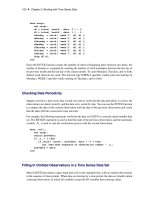
102 ✦ Chapter 3: Working with Time Series Data
data uscpi;
set uscpi;
d0 = intnx( 'month', date, 0 ) - 1;
d1 = intnx( 'month', date, 1 ) - 1;
nSunday = intck( 'week.1', d0, d1 );
nMonday = intck( 'week.2', d0, d1 );
nTuesday = intck( 'week.3', d0, d1 );
nWedday = intck( 'week.4', d0, d1 );
nThurday = intck( 'week.5', d0, d1 );
nFriday = intck( 'week.6', d0, d1 );
nSatday = intck( 'week.7', d0, d1 );
drop d0 d1;
run;
Since the INTCK function counts the number of interval beginning dates between two dates, the
number of Sundays is computed by counting the number of week boundaries between the last day of
the previous month and the last day of the current month. To count Mondays, Tuesdays, and so forth,
shifted week intervals are used. The interval type WEEK.2 specifies weekly intervals starting on
Mondays, WEEK.3 specifies weeks starting on Tuesdays, and so forth.
Checking Data Periodicity
Suppose you have a time series data set and you want to verify that the data periodicity is correct, the
observations are dated correctly, and the data set is sorted by date. You can use the INTCK function
to compare the date of the current observation with the date of the previous observation and verify
that the dates fall into consecutive time intervals.
For example, the following statements verify that the data set USCPI is a correctly dated monthly data
set. The RETAIN statement is used to hold the date of the previous observation, and the automatic
variable _N_ is used to start the verification process with the second observation.
data _null_;
set uscpi;
retain prevdate;
if _n_ > 1 then
if intck( 'month', prevdate, date ) ^= 1 then
put "Bad date sequence at observation number " _n_;
prevdate = date;
run;
Filling In Omitted Observations in a Time Series Data Set
Most SAS/ETS procedures expect input data to be in the standard form, with no omitted observations
in the sequence of time periods. When data are missing for a time period, the data set should contain
a missing observation, in which all variables except the ID variables have missing values.
Using Interval Functions for Calendar Calculations ✦ 103
You can replace omitted observations in a time series data set with missing observations with the
EXPAND procedure.
The following statements create a monthly data set, OMITTED, from data lines that contain records
for an intermittent sample of months. (Data values are not shown.) The OMITTED data set is sorted
to make sure it is in time order.
data omitted;
input date : monyy7. x y z;
format date monyy7.;
datalines;
jan1991
mar1991
apr1991
jun1991
etc.
;
proc sort data=omitted;
by date;
run;
This data set is converted to a standard form time series data set by the following PROC EXPAND
step. The TO= option specifies that monthly data is to be output, while the METHOD=NONE option
specifies that no interpolation is to be performed, so that the variables X, Y, and Z in the output
data set STANDARD will have missing values for the omitted time periods that are filled in by the
EXPAND procedure.
proc expand data=omitted
out=standard
to=month
method=none;
id date;
run;
Using Interval Functions for Calendar Calculations
With a little thought, you can come up with a formula that involves INTNX and INTCK functions
and different interval types to perform almost any calendar calculation.
For example, suppose you want to know the date of the third Wednesday in the month of October
1991. The answer can be computed as
intnx( 'week.4', '1oct91'd - 1, 3 )
which returns the SAS date value ’16OCT91’D.
104 ✦ Chapter 3: Working with Time Series Data
Consider this more complex example: how many weekdays are there between 17 October 1991
and the second Friday in November 1991, inclusive? The following formula computes the number
of weekdays between the date value contained in the variable DATE and the second Friday of the
following month (including the ending dates of this period):
n = intck( 'weekday', date - 1,
intnx( 'week.6', intnx( 'month', date, 1 ) - 1, 2 ) + 1 );
Setting DATE to ’17OCT91’D and applying this formula produces the answer, N=17.
Lags, Leads, Differences, and Summations
When working with time series data, you sometimes need to refer to the values of a series in previous
or future periods. For example, the usual interest in the consumer price index series shown in
previous examples is how fast the index is changing, rather than the actual level of the index. To
compute a percent change, you need both the current and the previous values of the series. When
you model a time series, you might want to use the previous values of other series as explanatory
variables.
This section discusses how to use the DATA step to perform operations over time: lags, differences,
leads, summations over time, and percent changes.
The EXPAND procedure can also be used to perform many of these operations; see Chapter 14, “The
EXPAND Procedure,” for more information. See also the section “Transforming Time Series” on
page 113.
The LAG and DIF Functions
The DATA step provides two functions, LAG and DIF, for accessing previous values of a variable or
expression. These functions are useful for computing lags and differences of series.
For example, the following statements add the variables CPILAG and CPIDIF to the USCPI data set.
The variable CPILAG contains lagged values of the CPI series. The variable CPIDIF contains the
changes of the CPI series from the previous period; that is, CPIDIF is CPI minus CPILAG. The new
data set is shown in part in Figure 3.16.
data uscpi;
set uscpi;
cpilag = lag( cpi );
cpidif = dif( cpi );
run;
proc print data=uscpi;
The LAG and DIF Functions ✦ 105
run;
Figure 3.16 USCPI Data Set with Lagged and Differenced Series
Plot of USCPI Data
Obs date cpi cpilag cpidif
1 JUN1990 129.9 . .
2 JUL1990 130.4 129.9 0.5
3 AUG1990 131.6 130.4 1.2
4 SEP1990 132.7 131.6 1.1
5 OCT1990 133.5 132.7 0.8
6 NOV1990 133.8 133.5 0.3
7 DEC1990 133.8 133.8 0.0
8 JAN1991 134.6 133.8 0.8
9 FEB1991 134.8 134.6 0.2
10 MAR1991 135.0 134.8 0.2
11 APR1991 135.2 135.0 0.2
12 MAY1991 135.6 135.2 0.4
13 JUN1991 136.0 135.6 0.4
14 JUL1991 136.2 136.0 0.2
Understanding the DATA Step LAG and DIF Functions
When used in this simple way, LAG and DIF act as lag and difference functions. However, it is
important to keep in mind that, despite their names, the LAG and DIF functions available in the
DATA step are not true lag and difference functions.
Rather, LAG and DIF are queuing functions that remember and return argument values from previous
calls. The LAG function remembers the value you pass to it and returns as its result the value you
passed to it on the previous call. The DIF function works the same way but returns the difference
between the current argument and the remembered value. (LAG and DIF return a missing value the
first time the function is called.)
A true lag function does not return the value of the argument for the “previous call,” as do the DATA
step LAG and DIF functions. Instead, a true lag function returns the value of its argument for the
“previous observation,” regardless of the sequence of previous calls to the function. Thus, for a true
lag function to be possible, it must be clear what the “previous observation” is.
If the data are sorted chronologically, then LAG and DIF act as true lag and difference functions. If
in doubt, use PROC SORT to sort your data before using the LAG and DIF functions. Beware of
missing observations, which can cause LAG and DIF to return values that are not the actual lag and
difference values.
The DATA step is a powerful tool that can read any number of observations from any number of
input files or data sets, can create any number of output data sets, and can write any number of
output observations to any of the output data sets, all in the same program. Thus, in general, it is not
clear what “previous observation” means in a DATA step program. In a DATA step program, the
“previous observation” exists only if you write the program in a simple way that makes this concept
meaningful.
106 ✦ Chapter 3: Working with Time Series Data
Since, in general, the previous observation is not clearly defined, it is not possible to make true lag
or difference functions for the DATA step. Instead, the DATA step provides queuing functions that
make it easy to compute lags and differences.
Pitfalls of DATA Step LAG and DIF Functions
The LAG and DIF functions compute lags and differences provided that the sequence of calls to the
function corresponds to the sequence of observations in the output data set. However, any complexity
in the DATA step that breaks this correspondence causes the LAG and DIF functions to produce
unexpected results.
For example, suppose you want to add the variable CPILAG to the USCPI data set, as in the previous
example, and you also want to subset the series to 1991 and later years. You might use the following
statements:
data subset;
set uscpi;
if date >= '1jan1991'd;
cpilag = lag( cpi ); /
*
WRONG PLACEMENT!
*
/
run;
If the subsetting IF statement comes before the LAG function call, the value of CPILAG will be
missing for January 1991, even though a value for December 1990 is available in the USCPI data
set. To avoid losing this value, you must rearrange the statements to ensure that the LAG function is
actually executed for the December 1990 observation.
data subset;
set uscpi;
cpilag = lag( cpi );
if date >= '1jan1991'd;
run;
In other cases, the subsetting statement should come before the LAG and DIF functions. For example,
the following statements subset the FOREOUT data set shown in a previous example to select only
_TYPE_=RESIDUAL observations and also to compute the variable LAGRESID:
data residual;
set foreout;
if _type_ = "RESIDUAL";
lagresid = lag( cpi );
run;
Another pitfall of LAG and DIF functions arises when they are used to process time series cross-
sectional data sets. For example, suppose you want to add the variable CPILAG to the CPICITY
data set shown in a previous example. You might use the following statements:
data cpicity;
set cpicity;
cpilag = lag( cpi );
run;
The LAG and DIF Functions ✦ 107
However, these statements do not yield the desired result. In the data set produced by these statements,
the value of CPILAG for the first observation for the first city is missing (as it should be), but in the
first observation for all later cities, CPILAG contains the last value for the previous city. To correct
this, set the lagged variable to missing at the start of each cross section, as follows:
data cpicity;
set cpicity;
by city date;
cpilag = lag( cpi );
if first.city then cpilag = .;
run;
Alternatives to LAG and DIF Functions
You can also use the EXPAND procedure to compute lags and differences. For example, the following
statements compute lag and difference variables for CPI:
proc expand data=uscpi out=uscpi method=none;
id date;
convert cpi=cpilag / transform=( lag 1 );
convert cpi=cpidif / transform=( dif 1 );
run;
You can also calculate lags and differences in the DATA step without using LAG and DIF functions.
For example, the following statements add the variables CPILAG and CPIDIF to the USCPI data set:
data uscpi;
set uscpi;
retain cpilag;
cpidif = cpi - cpilag;
output;
cpilag = cpi;
run;
The RETAIN statement prevents the DATA step from reinitializing CPILAG to a missing value at
the start of each iteration and thus allows CPILAG to retain the value of CPI assigned to it in the last
statement. The OUTPUT statement causes the output observation to contain values of the variables
before CPILAG is reassigned the current value of CPI in the last statement. This is the approach that
must be used if you want to build a variable that is a function of its previous lags.
LAG and DIF Functions in PROC MODEL
The preceding discussion of LAG and DIF functions applies to LAG and DIF functions available in
the DATA step. However, LAG and DIF functions are also used in the MODEL procedure.
The MODEL procedure LAG and DIF functions do not work like the DATA step LAG and DIF
functions. The LAG and DIF functions supported by PROC MODEL are true lag and difference
functions, not queuing functions.
108 ✦ Chapter 3: Working with Time Series Data
Unlike the DATA step, the MODEL procedure processes observations from a single input data set,
so the “previous observation” is always clearly defined in a PROC MODEL program. Therefore,
PROC MODEL is able to define LAG and DIF as true lagging functions that operate on values from
the previous observation. See Chapter 18, “The MODEL Procedure,” for more information about
LAG and DIF functions in the MODEL procedure.
Multiperiod Lags and Higher-Order Differencing
To compute lags at a lagging period greater than 1, add the lag length to the end of the LAG keyword
to specify the lagging function needed. For example, the LAG2 function returns the value of its
argument two calls ago, the LAG3 function returns the value of its argument three calls ago, and so
forth.
To compute differences at a lagging period greater than 1, add the lag length to the end of the DIF
keyword. For example, the DIF2 function computes the differences between the value of its argument
and the value of its argument two calls ago. (The maximum lagging period is 100.)
The following statements add the variables CPILAG12 and CPIDIF12 to the USCPI data set.
CPILAG12 contains the value of CPI from the same month one year ago. CPIDIF12 contains the
change in CPI from the same month one year ago. (In this case, the first 12 values of CPILAG12 and
CPIDIF12 are missing.)
data uscpi;
set uscpi;
cpilag12 = lag12( cpi );
cpidif12 = dif12( cpi );
run;
To compute second differences, take the difference of the difference. To compute higher-order
differences, nest DIF functions to the order needed. For example, the following statements compute
the second difference of CPI:
data uscpi;
set uscpi;
cpi2dif = dif( dif( cpi ) );
run;
Multiperiod lags and higher-order differencing can be combined. For example, the following
statements compute monthly changes in the inflation rate, with inflation rate computed as percent
change in CPI from the same month one year ago:
data uscpi;
set uscpi;
infchng = dif( 100
*
dif12( cpi ) / lag12( cpi ) );
run;
Percent Change Calculations ✦ 109
Percent Change Calculations
There are several common ways to compute the percent change in a time series. This section
illustrates the use of LAG and DIF functions by showing SAS statements for various kinds of percent
change calculations.
Computing Period-to-Period Change
To compute percent change from the previous period, divide the difference of the series by the lagged
value of the series and multiply by 100.
data uscpi;
set uscpi;
pctchng = dif( cpi ) / lag( cpi )
*
100;
label pctchng = "Monthly Percent Change, At Monthly Rates";
run;
Often, changes from the previous period are expressed at annual rates. This is done by exponentiation
of the current-to-previous period ratio to the number of periods in a year and expressing the result as
a percent change. For example, the following statements compute the month-over-month change in
CPI as a percent change at annual rates:
data uscpi;
set uscpi;
pctchng = ( ( cpi / lag( cpi ) )
**
12 - 1 )
*
100;
label pctchng = "Monthly Percent Change, At Annual Rates";
run;
Computing Year-over-Year Change
To compute percent change from the same period in the previous year, use LAG and DIF functions
with a lagging period equal to the number of periods in a year. (For quarterly data, use LAG4 and
DIF4. For monthly data, use LAG12 and DIF12.)
For example, the following statements compute monthly percent change in CPI from the same month
one year ago:
data uscpi;
set uscpi;
pctchng = dif12( cpi ) / lag12( cpi )
*
100;
label pctchng = "Percent Change from One Year Ago";
run;
To compute year-over-year percent change measured at a given period within the year, subset the
series of percent changes from the same period in the previous year to form a yearly data set. Use
an IF or WHERE statement to select observations for the period within each year on which the
year-over-year changes are based.
110 ✦ Chapter 3: Working with Time Series Data
For example, the following statements compute year-over-year percent change in CPI from December
of the previous year to December of the current year:
data annual;
set uscpi;
pctchng = dif12( cpi ) / lag12( cpi )
*
100;
label pctchng = "Percent Change: December to December";
if month( date ) = 12;
format date year4.;
run;
Computing Percent Change in Yearly Averages
To compute changes in yearly averages, first aggregate the series to an annual series by using the
EXPAND procedure, and then compute the percent change of the annual series. (See Chapter 14,
“The EXPAND Procedure,” for more information about PROC EXPAND.)
For example, the following statements compute percent changes in the annual averages of CPI:
proc expand data=uscpi out=annual from=month to=year;
convert cpi / observed=average method=aggregate;
run;
data annual;
set annual;
pctchng = dif( cpi ) / lag( cpi )
*
100;
label pctchng = "Percent Change in Yearly Averages";
run;
It is also possible to compute percent change in the average over the most recent yearly span. For
example, the following statements compute monthly percent change in the average of CPI over the
most recent 12 months from the average over the previous 12 months:
data uscpi;
retain sum12 0;
drop sum12 ave12 cpilag12;
set uscpi;
sum12 = sum12 + cpi;
cpilag12 = lag12( cpi );
if cpilag12 ^= . then sum12 = sum12 - cpilag12;
if lag11( cpi ) ^= . then ave12 = sum12 / 12;
pctchng = dif12( ave12 ) / lag12( ave12 )
*
100;
label pctchng = "Percent Change in 12 Month Moving Ave.";
run;
This example is a complex use of LAG and DIF functions that requires care in handling the
initialization of the moving-window averaging process. The LAG12 of CPI is checked for missing
values to determine when more than 12 values have been accumulated, and older values must be
removed from the moving sum. The LAG11 of CPI is checked for missing values to determine when
at least 12 values have been accumulated; AVE12 will be missing when LAG11 of CPI is missing.
The DROP statement prevents temporary variables from being added to the data set.
Leading Series ✦ 111
Note that the DIF and LAG functions must execute for every observation, or the queues of remem-
bered values will not operate correctly. The CPILAG12 calculation must be separate from the IF
statement. The PCTCHNG calculation must not be conditional on the IF statement.
The EXPAND procedure provides an alternative way to compute moving averages.
Leading Series
Although the SAS System does not provide a function to look ahead at the “next” value of a series,
there are a couple of ways to perform this task.
The most direct way to compute leads is to use the EXPAND procedure. For example:
proc expand data=uscpi out=uscpi method=none;
id date;
convert cpi=cpilead1 / transform=( lead 1 );
convert cpi=cpilead2 / transform=( lead 2 );
run;
Another way to compute lead series in SAS software is by lagging the time ID variable, renaming
the series, and merging the result data set back with the original data set.
For example, the following statements add the variable CPILEAD to the USCPI data set. The
variable CPILEAD contains the value of CPI in the following month. (The value of CPILEAD is
missing for the last observation, of course.)
data temp;
set uscpi;
keep date cpi;
rename cpi = cpilead;
date = lag( date );
if date ^= .;
run;
data uscpi;
merge uscpi temp;
by date;
run;
To compute leads at different lead lengths, you must create one temporary data set for each lead
length. For example, the following statements compute CPILEAD1 and CPILEAD2, which contain
leads of CPI for 1 and 2 periods, respectively:
data temp1(rename=(cpi=cpilead1))
temp2(rename=(cpi=cpilead2));
set uscpi;
keep date cpi;
date = lag( date );
if date ^= . then output temp1;
date = lag( date );

