SAS/ETS 9.22 User''''s Guide 31 ppt

292 ✦ Chapter 7: The ARIMA Procedure
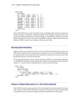
Output 7.2.8 Plot of the Forecast for the Original Series
Example 7.3: Model for Series J Data from Box and Jenkins
This example uses the Series J data from Box and Jenkins (1976). First, the input series X is modeled
with a univariate ARMA model. Next, the dependent series Y is cross-correlated with the input
series. Since a model has been fit to X, both Y and X are prewhitened by this model before the sample
cross-correlations are computed. Next, a transfer function model is fit with no structure on the noise
term. The residuals from this model are analyzed; then, the full model, transfer function and noise, is
fit to the data.
The following statements read
'Input Gas Rate'
and
'Output CO
2
'
from a gas furnace.
(Data values are not shown. The full example including data is in the SAS/ETS sample library.)
title1 'Gas Furnace Data';
title2 '(Box and Jenkins, Series J)';
data seriesj;
input x y @@;
label x = 'Input Gas Rate'
y = 'Output CO2';
Example 7.3: Model for Series J Data from Box and Jenkins ✦ 293
datalines;
more lines
The following statements produce Output 7.3.1 through Output 7.3.11:
ods graphics on;
proc arima data=seriesj;
/
*

Look at the input process
*
/
identify var=x;
run;
/
*
Fit a model for the input
*
/
estimate p=3 plot;
run;
/
*
Crosscorrelation of prewhitened series
*
/
identify var=y crosscorr=(x) nlag=12;
run;
/
*
- Fit a simple transfer function - look at residuals -
*
/
estimate input=( 3 $ (1,2)/(1) x );
run;
/
*
Final Model - look at residuals
*

/
estimate p=2 input=( 3 $ (1,2)/(1) x );
run;
quit;
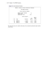
The results of the first IDENTIFY statement for the input series X are shown in Output 7.3.1. The
correlation analysis suggests an AR(3) model.
Output 7.3.1 IDENTIFY Statement Results for X
Gas Furnace Data
(Box and Jenkins, Series J)
The ARIMA Procedure
Name of Variable = x
Mean of Working Series -0.05683
Standard Deviation 1.070952
Number of Observations 296
294 ✦ Chapter 7: The ARIMA Procedure
Output 7.3.2 IDENTIFY Statement Results for X: Trend and Correlation
The ESTIMATE statement results for the AR(3) model for the input series X are shown in Out-
put 7.3.3.
Output 7.3.3 Estimates of the AR(3) Model for X
Conditional Least Squares Estimation
Standard Approx
Parameter Estimate Error t Value Pr > |t| Lag
MU -0.12280 0.10902 -1.13 0.2609 0
AR1,1 1.97607 0.05499 35.94 <.0001 1
AR1,2 -1.37499 0.09967 -13.80 <.0001 2
AR1,3 0.34336 0.05502 6.24 <.0001 3
Constant Estimate -0.00682
Variance Estimate 0.035797
Std Error Estimate 0.1892
AIC -141.667

SBC -126.906
Number of Residuals 296
Example 7.3: Model for Series J Data from Box and Jenkins ✦ 295
Output 7.3.3 continued
Model for variable x
Estimated Mean -0.1228
Autoregressive Factors
Factor 1: 1 - 1.97607 B
**
(1) + 1.37499 B
**
(2) - 0.34336 B
**
(3)
The IDENTIFY statement results for the dependent series Y cross-correlated with the input series X
are shown in Output 7.3.4, Output 7.3.5, Output 7.3.6, and Output 7.3.7. Since a model has been fit
to X, both Y and X are prewhitened by this model before the sample cross-correlations are computed.
Output 7.3.4 Summary Table: Y Cross-Correlated with X
Correlation of y and x
Number of Observations 296
Variance of transformed series y 0.131438
Variance of transformed series x 0.035357
Both series have been prewhitened.
Output 7.3.5 Prewhitening Filter
Autoregressive Factors
Factor 1: 1 - 1.97607 B
**
(1) + 1.37499 B
**
(2) - 0.34336 B

**
(3)
296 ✦ Chapter 7: The ARIMA Procedure
Output 7.3.6 IDENTIFY Statement Results for Y: Trend and Correlation
Example 7.3: Model for Series J Data from Box and Jenkins ✦ 297
Output 7.3.7 IDENTIFY Statement for Y Cross-Correlated with X
The ESTIMATE statement results for the transfer function model with no structure on the noise term
are shown in Output 7.3.8, Output 7.3.9, and Output 7.3.10.
Output 7.3.8 Estimation Output of the First Transfer Function Model
Conditional Least Squares Estimation
Standard Approx
Parameter Estimate Error t Value Pr > |t| Lag Variable Shift
MU 53.32256 0.04926 1082.51 <.0001 0 y 0
NUM1 -0.56467 0.22405 -2.52 0.0123 0 x 3
NUM1,1 0.42623 0.46472 0.92 0.3598 1 x 3
NUM1,2 0.29914 0.35506 0.84 0.4002 2 x 3
DEN1,1 0.60073 0.04101 14.65 <.0001 1 x 3
Constant Estimate 53.32256
Variance Estimate 0.702625
Std Error Estimate 0.838227
AIC 728.0754
SBC 746.442
Number of Residuals 291
298 ✦ Chapter 7: The ARIMA Procedure
Output 7.3.9 Model Summary: First Transfer Function Model
Model for variable y
Estimated Intercept 53.32256
Input Number 1
Input Variable x
Shift 3

Numerator Factors
Factor 1: -0.5647 - 0.42623 B
**
(1) - 0.29914 B
**
(2)
Denominator Factors
Factor 1: 1 - 0.60073 B
**
(1)
Output 7.3.10 Residual Analysis: First Transfer Function Model
Example 7.3: Model for Series J Data from Box and Jenkins ✦ 299
The residual correlation analysis suggests an AR(2) model for the noise part of the model. The
ESTIMATE statement results for the final transfer function model with AR(2) noise are shown in
Output 7.3.11.
Output 7.3.11 Estimation Output of the Final Model
Conditional Least Squares Estimation
Standard Approx
Parameter Estimate Error t Value Pr > |t| Lag Variable Shift
MU 53.26304 0.11929 446.48 <.0001 0 y 0
AR1,1 1.53291 0.04754 32.25 <.0001 1 y 0
AR1,2 -0.63297 0.05006 -12.64 <.0001 2 y 0
NUM1 -0.53522 0.07482 -7.15 <.0001 0 x 3
NUM1,1 0.37603 0.10287 3.66 0.0003 1 x 3
NUM1,2 0.51895 0.10783 4.81 <.0001 2 x 3
DEN1,1 0.54841 0.03822 14.35 <.0001 1 x 3
Constant Estimate 5.329425
Variance Estimate 0.058828
Std Error Estimate 0.242544
AIC 8.292809

SBC 34.00607
Number of Residuals 291
300 ✦ Chapter 7: The ARIMA Procedure
Output 7.3.12 Residual Analysis of the Final Model
Output 7.3.13 Model Summary of the Final Model
Model for variable y
Estimated Intercept 53.26304
Autoregressive Factors
Factor 1: 1 - 1.53291 B
**
(1) + 0.63297 B
**
(2)
Input Number 1
Input Variable x
Shift 3
Numerator Factors
Factor 1: -0.5352 - 0.37603 B
**
(1) - 0.51895 B
**
(2)
Denominator Factors
Factor 1: 1 - 0.54841 B
**
(1)
Example 7.4: An Intervention Model for Ozone Data ✦ 301
Example 7.4: An Intervention Model for Ozone Data
This example fits an intervention model to ozone data as suggested by Box and Tiao (1975). Notice
that the response variable, OZONE, and the innovation, X1, are seasonally differenced. The final

model for the differenced data is a multiple regression model with a moving-average structure
assumed for the residuals.
The model is fit by maximum likelihood. The seasonal moving-average parameter and its standard
error are fairly sensitive to which method is chosen to fit the model, in agreement with the observations
of Davidson (1981) and Ansley and Newbold (1980); thus, fitting the model by the unconditional or
conditional least squares method produces somewhat different estimates for these parameters.
Some missing values are appended to the end of the input data to generate additional values for
the independent variables. Since the independent variables are not modeled, values for them must
be available for any times at which predicted values are desired. In this case, predicted values are
requested for 12 periods beyond the end of the data. Thus, values for X1, WINTER, and SUMMER
must be given for 12 periods ahead.
The following statements read in the data and compute dummy variables for use as intervention
inputs:
title1 'Intervention Data for Ozone Concentration';
title2 '(Box and Tiao, JASA 1975 P.70)';
data air;
input ozone @@;
label ozone = 'Ozone Concentration'
x1 = 'Intervention for post 1960 period'
summer = 'Summer Months Intervention'
winter = 'Winter Months Intervention';
date = intnx( 'month', '31dec1954'd, _n_ );
format date monyy.;
month = month( date );
year = year( date );
x1 = year >= 1960;
summer = ( 5 < month < 11 )
*
( year > 1965 );
winter = ( year > 1965 ) - summer;

datalines;
2.7 2.0 3.6 5.0 6.5 6.1 5.9 5.0 6.4 7.4 8.2 3.9
4.1 4.5 5.5 3.8 4.8 5.6 6.3 5.9 8.7 5.3 5.7 5.7
3.0 3.4 4.9 4.5 4.0 5.7 6.3 7.1 8.0 5.2 5.0 4.7
more lines
The following statements produce Output 7.4.1 through Output 7.4.3: