SAS/ETS 9.22 User''''s Guide 88 ppt

862 ✦ Chapter 15: The FORECAST Procedure
Output 15.2.2 Nondurable Goods Sales
The following statements produce the forecast:
title1 "Forecasting Sales of Durable and Nondurable Goods";
proc forecast data=sashelp.usecon interval=month
method=stepar trend=2 lead=12
out=out outfull outest=est;
id date;
var durables nondur;
where date >= '1jan80'd;
run;
The following statements print the OUTEST= data set.
title2 'OUTEST= Data Set: STEPAR Method';
proc print data=est;
run;
The PROC PRINT listing of the OUTEST= data set is shown in Output 15.2.3.
Example 15.2: Forecasting Retail Sales ✦ 863
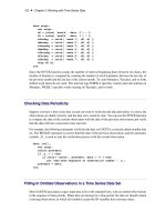
Output 15.2.3 The OUTEST= Data Set Produced by PROC FORECAST
Forecasting Sales of Durable and Nondurable Goods
OUTEST= Data Set: STEPAR Method
Obs _TYPE_ DATE DURABLES NONDUR
1 N DEC91 144 144
2 NRESID DEC91 144 144
3 DF DEC91 137 139
4 SIGMA DEC91 4519.451 2452.2642
5 CONSTANT DEC91 71884.597 73190.812
6 LINEAR DEC91 400.90106 308.5115
7 AR01 DEC91 0.5844515 0.8243265
8 AR02 DEC91 . .
9 AR03 DEC91 . .
10 AR04 DEC91 . .

11 AR05 DEC91 . .
12 AR06 DEC91 0.2097977 .
13 AR07 DEC91 . .
14 AR08 DEC91 . .
15 AR09 DEC91 . .
16 AR10 DEC91 -0.119425 .
17 AR11 DEC91 . .
18 AR12 DEC91 0.6138699 0.8050854
19 AR13 DEC91 -0.556707 -0.741854
20 SST DEC91 4.923E10 2.8331E10
21 SSE DEC91 1.88157E9 544657337
22 MSE DEC91 13734093 3918398.1
23 RMSE DEC91 3705.9538 1979.4944
24 MAPE DEC91 2.9252601 1.6555935
25 MPE DEC91 -0.253607 -0.085357
26 MAE DEC91 2866.675 1532.8453
27 ME DEC91 -67.87407 -29.63026
28 RSQUARE DEC91 0.9617803 0.9807752
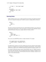
The following statements plot the forecasts and confidence limits. The last two years of historical
data are included in the plots to provide context for the forecast. A reference line is drawn at the start
of the forecast period.
title1 'Plot of Forecasts from STEPAR Method';
proc sgplot data=out;
series x=date y=durables / group=_type_;
xaxis values=('1jan90'd to '1jan93'd by qtr);
yaxis values=(100000 to 150000 by 10000);
refline '15dec91'd / axis=x;
run;
proc sgplot data=out;
series x=date y=nondur / group=_type_;

xaxis values=('1jan90'd to '1jan93'd by qtr);
yaxis values=(100000 to 140000 by 10000);
refline '15dec91'd / axis=x;
run;
864 ✦ Chapter 15: The FORECAST Procedure
The plots are shown in Output 15.2.4 and Output 15.2.5.
Output 15.2.4 Forecast of Durable Goods Sales
Example 15.3: Forecasting Petroleum Sales ✦ 865
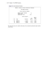
Output 15.2.5 Forecast of Nondurable Goods Sales
Example 15.3: Forecasting Petroleum Sales
This example uses the double exponential smoothing method to forecast the monthly U. S. sales of
petroleum and related products series (PETROL) from the data set SASHELP.USECON. These data
are taken from Business Statistics, published by the U.S. Bureau of Economic Analysis.
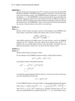
The following statements plot the PETROL series:
title1 "Sales of Petroleum and Related Products";
proc sgplot data=sashelp.usecon;
series x=date y=petrol / markers;
xaxis values=('1jan80'd to '1jan92'd by year);
yaxis values=(8000 to 20000 by 1000);
format date year4.;
run;
The plot is shown in Output 15.3.1.
866 ✦ Chapter 15: The FORECAST Procedure
Output 15.3.1 Sales of Petroleum and Related Products
The following statements produce the forecast:
proc forecast data=sashelp.usecon interval=month
method=expo trend=2 lead=12
out=out outfull outest=est;
id date;
var petrol;

where date >= '1jan80'd;
run;
The following statements print the OUTEST= data set:
title2 'OUTEST= Data Set: EXPO Method';
proc print data=est;
run;
The PROC PRINT listing of the output data set is shown in Output 15.3.2.
Example 15.3: Forecasting Petroleum Sales ✦ 867
Output 15.3.2 The OUTEST= Data Set Produced by PROC FORECAST
Sales of Petroleum and Related Products
OUTEST= Data Set: EXPO Method
Obs _TYPE_ DATE PETROL
1 N DEC91 144
2 NRESID DEC91 144
3 DF DEC91 142
4 WEIGHT DEC91 0.1055728
5 S1 DEC91 14165.259
6 S2 DEC91 13933.435
7 SIGMA DEC91 1281.0945
8 CONSTANT DEC91 14397.084
9 LINEAR DEC91 27.363164
10 SST DEC91 1.17001E9
11 SSE DEC91 233050838
12 MSE DEC91 1641203.1
13 RMSE DEC91 1281.0945
14 MAPE DEC91 6.5514467
15 MPE DEC91 -0.147168
16 MAE DEC91 891.04243
17 ME DEC91 8.2148584
18 RSQUARE DEC91 0.8008122

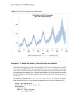
The plot of the forecast is shown in Output 15.3.3.
title1 "Sales of Petroleum and Related Products";
title2 'Plot of Forecast: EXPO Method';
proc sgplot data=out;
series x=date y=petrol / group=_type_;
xaxis values=('1jan89'd to '1jan93'd by qtr);
yaxis values=(10000 to 20000 by 1000);
refline '15dec91'd / axis=x;
run;
868 ✦ Chapter 15: The FORECAST Procedure
Output 15.3.3 Forecast of Petroleum and Related Products
References
Ahlburg, D. A. (1984). “Forecast Evaluation and Improvement Using Theil’s Decomposition,”
Journal of Forecasting, 3, 345–351.
Aldrin, M. and Damsleth, E. (1989). “Forecasting Non-Seasonal Time Series with Missing Observa-
tions,” Journal of Forecasting, 8, 97–116.
Archibald, B.C. (1990), “Parameter Space of the Holt-Winters’ Model,” International Journal of
Forecasting, 6, 199–209.
Bails, D.G. and Peppers, L.C. (1982), Business Fluctuations: Forecasting Techniques and Applica-
tions, New Jersey: Prentice-Hall.
Bartolomei, S.M. and Sweet, A.L. (1989). “A Note on the Comparison of Exponential Smoothing
Methods for Forecasting Seasonal Series,” International Journal of Forecasting, 5, 111–116.
Bureau of Economic Analysis, U.S. Department of Commerce (1992 and earlier editions), Business
References ✦ 869
Statistics, 27th and earlier editions, Washington: U.S. Government Printing Office.
Bliemel, F. (1973). “Theil’s Forecast Accuracy Coefficient: A Clarification,” Journal of Marketing
Research, 10, 444–446.
Bowerman, B.L. and O’Connell, R.T. (1979), Time Series and Forecasting: An Applied Approach,
North Scituate, Massachusetts: Duxbury Press.
Box, G.E.P. and Jenkins, G.M. (1976), Time Series Analysis: Forecasting and Control, Revised

Edition, San Francisco: Holden-Day.
Bretschneider, S.I., Carbone, R., and Longini, R.L. (1979). “An Adaptive Approach to Time Series
Forecasting,” Decision Sciences, 10, 232–244.
Brown, R.G. (1962), Smoothing, Forecasting and Prediction of Discrete Time Series, New York:
Prentice-Hall.
Brown, R.G. and Meyer, R.F. (1961). “The Fundamental Theorem of Exponential Smoothing,”
Operations Research, 9, 673–685.
Chatfield, C. (1978). “The Holt-Winters Forecasting Procedure,” Applied Statistics, 27, 264–279.
Chatfield, C., and Prothero, D.L. (1973). “Box-Jenkins Seasonal Forecasting: Problems in a Case
Study,” Journal of the Royal Statistical Society, Series A, 136, 295–315.
Chow, W.M. (1965). “Adaptive Control of the Exponential Smoothing Constant,” Journal of
Industrial Engineering, September–October 1965.
Cogger, K.O. (1974). “The Optimality of General-Order Exponential Smoothing,” Operations
Research, 22, 858–.
Cox, D. R. (1961). “Prediction by Exponentially Weighted Moving Averages and Related Methods,”
Journal of the Royal Statistical Society, Series B, 23, 414–422.
Fair, R.C. (1986). “Evaluating the Predictive Accuracy of Models,” In Handbook of Econometrics,
Vol. 3., Griliches, Z. and Intriligator, M.D., eds. New York: North Holland.
Fildes, R. (1979). “Quantitative Forecasting—The State of the Art: Extrapolative Models,” Journal
of Operational Research Society, 30, 691–710.
Gardner, E.S. (1984). “The Strange Case of the Lagging Forecasts,” Interfaces, 14, 47–50.
Gardner, E.S., Jr. (1985). “Exponential Smoothing: The State of the Art,” Journal of Forecasting, 4,
1–38.
Granger, C.W.J. and Newbold, P. (1977), Forecasting Economic Time Series, New York: Academic
Press, Inc.
Harvey, A.C. (1984). “A Unified View of Statistical Forecasting Procedures,” Journal of Forecasting,
3, 245–275.
870 ✦ Chapter 15: The FORECAST Procedure
Ledolter, J. and Abraham, B. (1984). “Some Comments on the Initialization of Exponential Smooth-
ing,” Journal of Forecasting, 3, 79–84.

Maddala, G.S. (1977), Econometrics, New York: McGraw-Hill.
Makridakis, S., Wheelwright, S.C., and McGee, V.E. (1983). Forecasting: Methods and Applications,
2nd Ed. New York: John Wiley and Sons.
McKenzie, Ed (1984). “General Exponential Smoothing and the Equivalent ARMA Process,” Journal
of Forecasting, 3, 333–344.
Montgomery, D.C. and Johnson, L.A. (1976), Forecasting and Time Series Analysis, New York:
McGraw-Hill.
Muth, J.F. (1960). “Optimal Properties of Exponentially Weighted Forecasts,” Journal of the
American Statistical Association, 55, 299–306.
Pierce, D.A. (1979). “
R
2
Measures for Time Series,” Journal of the American Statistical Association,
74, 901–910.
Pindyck, R.S. and Rubinfeld, D.L. (1981), Econometric Models and Economic Forecasts, Second
Edition, New York: McGraw-Hill.
Raine, J.E. (1971). “Self-Adaptive Forecasting Reconsidered,” Decision Sciences, 2, 181–191.
Roberts, S.A. (1982). “A General Class of Holt-Winters Type Forecasting Models,” Management
Science, 28, 808–820.
Theil, H. (1966). Applied Economic Forecasting. Amsterdam: North Holland.
Trigg, D.W., and Leach, A.G. (1967). “Exponential Smoothing with an Adaptive Response Rate,”
Operational Research Quarterly, 18, 53–59.
Winters, P.R. (1960). “Forecasting Sales by Exponentially Weighted Moving Averages,” Management
Science, 6, 324–342.
Chapter 16
The LOAN Procedure
Contents
Overview: LOAN Procedure . . . . . . . . . . . . . . . . . . . . . . . . . . . . . 872
Getting Started: LOAN Procedure . . . . . . . . . . . . . . . . . . . . . . . . . . 872
Analyzing Fixed Rate Loans . . . . . . . . . . . . . . . . . . . . . . . . . . 873

Analyzing Balloon Payment Loans . . . . . . . . . . . . . . . . . . . . . . 874
Analyzing Adjustable Rate Loans . . . . . . . . . . . . . . . . . . . . . . . 875
Analyzing Buydown Rate Loans . . . . . . . . . . . . . . . . . . . . . . . . 876
Loan Repayment Schedule . . . . . . . . . . . . . . . . . . . . . . . . . . . . 877
Loan Comparison . . . . . . . . . . . . . . . . . . . . . . . . . . . . . . . 879
Syntax: LOAN Procedure . . . . . . . . . . . . . . . . . . . . . . . . . . . . . . 882
Functional Summary . . . . . . . . . . . . . . . . . . . . . . . . . . . . . . 882
PROC LOAN Statement . . . . . . . . . . . . . . . . . . . . . . . . . . . . 884
FIXED Statement . . . . . . . . . . . . . . . . . . . . . . . . . . . . . . . 885
BALLOON Statement . . . . . . . . . . . . . . . . . . . . . . . . . . . . . 889
ARM Statement . . . . . . . . . . . . . . . . . . . . . . . . . . . . . . . . 889
BUYDOWN Statement . . . . . . . . . . . . . . . . . . . . . . . . . . . . 892
COMPARE Statement . . . . . . . . . . . . . . . . . . . . . . . . . . . . . 892
Details: LOAN Procedure . . . . . . . . . . . . . . . . . . . . . . . . . . . . . . 894
Computational Details . . . . . . . . . . . . . . . . . . . . . . . . . . . . . 894
Loan Comparison Details . . . . . . . . . . . . . . . . . . . . . . . . . . . 896
OUT= Data Set . . . . . . . . . . . . . . . . . . . . . . . . . . . . . . . . . . 897
OUTCOMP= Data Set . . . . . . . . . . . . . . . . . . . . . . . . . . . . . 898
OUTSUM= Data Set . . . . . . . . . . . . . . . . . . . . . . . . . . . . . . 898
Printed Output . . . . . . . . . . . . . . . . . . . . . . . . . . . . . . . . . 899
ODS Table Names . . . . . . . . . . . . . . . . . . . . . . . . . . . . . . . 900
Examples: LOAN Procedure . . . . . . . . . . . . . . . . . . . . . . . . . . . . . . 901
Example 16.1: Discount Points for Lower Interest Rates . . . . . . . . . . . . 901
Example 16.2: Refinancing a Loan . . . . . . . . . . . . . . . . . . . . . . 904
Example 16.3: Prepayments on a Loan . . . . . . . . . . . . . . . . . . . . 906
Example 16.4: Output Data Sets . . . . . . . . . . . . . . . . . . . . . . . . 907
Example 16.5: Piggyback Loans . . . . . . . . . . . . . . . . . . . . . . . 910
References . . . . . . . . . . . . . . . . . . . . . . . . . . . . . . . . . . . . . . 912