SAS/ETS 9.22 User''''s Guide 172 ppt

1702 ✦ Chapter 25: The SPECTRA Procedure
Printed Output
By default PROC SPECTRA produces no printed output.
When the WHITETEST option is specified, the SPECTRA procedure prints the following statistics
for each variable in the VAR statement:
1. the name of the variable
2. M–1, the number of two-degree-of-freedom periodogram ordinates used in the test
3. MAX(P(*)), the maximum periodogram ordinate
4. SUM(P(*)), the sum of the periodogram ordinates
5. Fisher’s Kappa statistic
6. Bartlett’s Kolmogorov-Smirnov test statistic
7. Approximate p-value for Bartlett’s Kolmogorov-Smirnov test statistic
See the section “White Noise Test” on page 1699 for details.
ODS Table Names: SPECTRA procedure
PROC SPECTRA assigns a name to each table it creates. You can use these names to reference the
table when you use the Output Delivery System (ODS) to select tables and create output data sets.
These names are listed in the following table.
Table 25.4 ODS Tables Produced in PROC SPECTRA
ODS Table Name Description Option
WhiteNoiseTest white noise test WHITETEST
Kappa Fishers Kappa statistic WHITETEST
Bartlett Bartletts Kolmogorov-Smirnov statistic WHITETEST
Examples: SPECTRA Procedure ✦ 1703
Examples: SPECTRA Procedure
Example 25.1: Spectral Analysis of Sunspot Activity
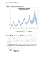
This example analyzes Wolfer’s sunspot data (Anderson 1971). The following statements read and
plot the data.
title "Wolfer's Sunspot Data";
data sunspot;
input year wolfer @@;
datalines;

more lines
proc sgplot data=sunspot;
series x=year y=wolfer / markers markerattrs=(symbol=circlefilled);
xaxis values=(1740 to 1930 by 10);
yaxis values=(0 to 1600 by 200);
run;
The plot of the sunspot series is shown in Output 25.1.1.
1704 ✦ Chapter 25: The SPECTRA Procedure
Output 25.1.1 Plot of Original Sunspot Data
The spectral analysis of the sunspot series is performed by the following statements:
proc spectra data=sunspot out=b p s adjmean whitetest;
var wolfer;
weights 1 2 3 4 3 2 1;
run;
proc print data=b(obs=12);
run;
The PROC SPECTRA statement specifies the P and S options to write the periodogram and spectral
density estimates to the OUT= data set B. The WEIGHTS statement specifies a triangular spectral
window for smoothing the periodogram to produce the spectral density estimate. The ADJMEAN
option zeros the frequency 0 value and avoids the need to exclude that observation from the plots.
The WHITETEST option prints tests for white noise.
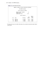
The Fisher’s Kappa test statistic of 16.070 is larger than the 5% critical value of 7.2, so the null
hypothesis that the sunspot series is white noise is rejected (see the table of critical values in Fuller
(1976)).
The Bartlett’s Kolmogorov-Smirnov statistic is 0.6501, and its approximate p-value is
< 0:0001
. The
small p-value associated with this test leads to the rejection of the null hypothesis that the spectrum
represents white noise.
Example 25.1: Spectral Analysis of Sunspot Activity ✦ 1705

The printed output produced by PROC SPECTRA is shown in Output 25.1.2. The output data set B
created by PROC SPECTRA is shown in part in Output 25.1.3.
Output 25.1.2 White Noise Test Results
Wolfer's Sunspot Data
The SPECTRA Procedure
Test for White Noise for Variable wolfer
M-1 87
Max(P(
*
)) 4062267
Sum(P(
*
)) 21156512
Fisher's Kappa: (M-1)
*
Max(P(
*
))/Sum(P(
*
))
Kappa 16.70489
Bartlett's Kolmogorov-Smirnov Statistic:
Maximum absolute difference of the standardized
partial sums of the periodogram and the CDF of a
uniform(0,1) random variable.
Test Statistic 0.650055
Approximate P-Value <.0001
Output 25.1.3 First 12 Observations of the OUT= Data Set
Wolfer's Sunspot Data
Obs FREQ PERIOD P_01 S_01

1 0.00000 . 0.00 59327.52
2 0.03570 176.000 3178.15 61757.98
3 0.07140 88.000 2435433.22 69528.68
4 0.10710 58.667 1077495.76 66087.57
5 0.14280 44.000 491850.36 53352.02
6 0.17850 35.200 2581.12 36678.14
7 0.21420 29.333 181163.15 20604.52
8 0.24990 25.143 283057.60 15132.81
9 0.28560 22.000 188672.97 13265.89
10 0.32130 19.556 122673.94 14953.32
11 0.35700 17.600 58532.93 16402.84
12 0.39270 16.000 213405.16 18562.13
The following statements plot the periodogram and spectral density estimate by the frequency and
period.
1706 ✦ Chapter 25: The SPECTRA Procedure
proc sgplot data=b;
series x=freq y=p_01 / markers markerattrs=(symbol=circlefilled);
run;
proc sgplot data=b;
series x=period y=p_01 / markers markerattrs=(symbol=circlefilled);
run;
proc sgplot data=b;
series x=freq y=s_01 / markers markerattrs=(symbol=circlefilled);
run;
proc sgplot data=b;
series x=period y=s_01 / markers markerattrs=(symbol=circlefilled);
run;
The periodogram is plotted against the frequency in Output 25.1.4 and plotted against the period in
Output 25.1.5. The spectral density estimate is plotted against the frequency in Output 25.1.6 and
plotted against the period in Output 25.1.7.

Output 25.1.4 Plot of Periodogram by Frequency
Example 25.1: Spectral Analysis of Sunspot Activity ✦ 1707
Output 25.1.5 Plot of Periodogram by Period
1708 ✦ Chapter 25: The SPECTRA Procedure
Output 25.1.6 Plot of Spectral Density Estimate by Frequency
Example 25.1: Spectral Analysis of Sunspot Activity ✦ 1709
Output 25.1.7 Plot of Spectral Density Estimate by Period
Since PERIOD is the reciprocal of frequency, the plot axis for PERIOD is stretched for low frequen-
cies and compressed at high frequencies. One way to correct for this is to use a WHERE statement
to restrict the plots and exclude the low frequency components. The following statements plot the
spectral density for periods less than 50.
proc sgplot data=b;
where period < 50;
series x=period y=s_01 / markers markerattrs=(symbol=circlefilled);
refline 11 / axis=x;
run;
title;
The spectral analysis of the sunspot series confirms a strong 11-year cycle of sunspot activity. The
plot makes this clear by drawing a reference line at the 11 year period, which highlights the position
of the main peak in the spectral density.
Output 25.1.8 shows the plot. Contrast Output 25.1.8 with Output 25.1.7.
1710 ✦ Chapter 25: The SPECTRA Procedure
Output 25.1.8 Plot of Spectral Density Estimate by Period to 50 Years
Example 25.2: Cross-Spectral Analysis
This example uses simulated data to show cross-spectral analysis for two variables X and Y. X is
generated by an AR(1) process; Y is generated as white noise plus an input from X lagged 2 periods.
All output options are specified in the PROC SPECTRA statement. PROC CONTENTS shows the
contents of the OUT= data set.
data a;
xl = 0; xll = 0;

do i = - 10 to 100;
x = .4
*
xl + rannor(123);
y = .5
*
xll + rannor(123);
if i > 0 then output;
xll = xl; xl = x;
end;
run;
Example 25.2: Cross-Spectral Analysis ✦ 1711
proc spectra data=a out=b cross coef a k p ph s;
var x y;
weights 1 1.5 2 4 8 9 8 4 2 1.5 1;
run;
proc contents data=b position;
run;
The PROC CONTENTS report for the output data set B is shown in Output 25.2.1.
Output 25.2.1 Contents of PROC SPECTRA OUT= Data Set
The CONTENTS Procedure
Alphabetic List of Variables and Attributes
# Variable Type Len Label
16 A_01_02 Num 8 Amplitude of x by y
3 COS_01 Num 8 Cosine Transform of x
5 COS_02 Num 8 Cosine Transform of y
13 CS_01_02 Num 8 Cospectra of x by y
1 FREQ Num 8 Frequency from 0 to PI
12 IP_01_02 Num 8 Imag Periodogram of x by y
15 K_01_02 Num 8 Coherency

**
2 of x by y
2 PERIOD Num 8 Period
17 PH_01_02 Num 8 Phase of x by y
7 P_01 Num 8 Periodogram of x
8 P_02 Num 8 Periodogram of y
14 QS_01_02 Num 8 Quadrature of x by y
11 RP_01_02 Num 8 Real Periodogram of x by y
4 SIN_01 Num 8 Sine Transform of x
6 SIN_02 Num 8 Sine Transform of y
9 S_01 Num 8 Spectral Density of x
10 S_02 Num 8 Spectral Density of y
The following statements plot the amplitude of the cross-spectrum estimate against frequency and
against period for periods less than 25.
proc sgplot data=b;
series x=freq y=a_01_02 / markers markerattrs=(symbol=circlefilled);
xaxis values=(0 to 4 by 1);
run;
The plot of the amplitude of the cross-spectrum estimate against frequency is shown in Output 25.2.2.