Character Animation with Direct3D- P8 potx
Bạn đang xem bản rút gọn của tài liệu. Xem và tải ngay bản đầy đủ của tài liệu tại đây (805.56 KB, 20 trang )
That’s pretty much all you need for a lightweight physics simulation. Note
that there are light-years between a physics engine like this and a proper engine.
For example, this “engine” doesn’t handle things like object–object collision, etc.
Next, you’ll learn how the position of an object is updated, and after that the first
physics object (the particle) will be implemented.
P
OSITION, VELOCITY, AND ACCELERATION
Next I’ll cover the three most basic physical properties of a rigid body: its position p,
its velocity v, and its acceleration a. In 3D space, the position of an object is described
with x, y, and z coordinates. The velocity of an object is simply how the position
is changing over time. In just the same way, the acceleration of an object is how the
velocity changes over time. The formulas for these behaviors are listed below.
p
n
= p + v • t
where p
n
is the new position.
v
n
= v + a • t
where v
n
is the new velocity.
a =
f
m
In the case of a 3D object, these are all described as a 3D vector with an x, y, and
z component. The following code shows an example class that has the
m_position,
m_velocity, and the m_acceleration vector. This class implements the formulas
above using a constant acceleration:
class OBJECT{
public:
OBJECT()
{
m_position = D3DXVECTOR3(0.0f, 0.0f, 0.0f);
m_velocity = D3DXVECTOR3(0.0f, 0.0f, 0.0f);
m_acceleration = D3DXVECTOR3(0.0f, 1.0f, 0.0f);
}
void Update(float deltaTime)
{
126 Character Animation with Direct3D
ٌ
ٌ
Please purchase PDF Split-Merge on www.verypdf.com to remove this watermark.
m_velocity += m_acceleration * deltaTime;
m_position += m_velocity * deltaTime;
}
private:
D3DXVECTOR3 m_position;
D3DXVECTOR3 m_velocity;
D3DXVECTOR3 m_acceleration;
};
As you can see, the m_position and the m_velocity vectors are initialized to
zero, while the
m_acceleration vector is pointing in the Y-direction with a constant
magnitude of one. Figure 6.11 shows a graph of how the acceleration, velocity, and
position of an object like this change over time.
In this section you have looked at how an object’s position is affected by
velocity, which in turn is affected by its acceleration. In the same manner, an
object’s orientation is affected by its angular velocity, which in turn is affected by
its torque. However, since you won’t need the concepts of angular velocity and
torque to create a simple ragdoll animation, I won’t dive into the detailed math
of these. If you want to look into the specifics of angular velocity and torque, I
suggest reading the article “Integrating the Equations of Rigid Body Motion” by
Miguel Gomez [Gomez00].
T
HE PARTICLE
These days, physicists use billions of volts to try and accelerate tiny electrically
charged particles and collide them with each other. What you’re about to engage in
is, thankfully, much simpler than that (and also a lot less expensive). You’ll be
looking at the smallest (and simplest) entity you can simulate in a physics engine:
the particle!
Chapter 6 Physics Primer 127
FIGURE 6.11
Acceleration, velocity, and position over time.
Please purchase PDF Split-Merge on www.verypdf.com to remove this watermark.
A particle can have a mass, but it does not have a volume and therefore it
doesn’t have an orientation either. This makes it a perfect physical entity for us
beginners to start with. The particle system I am about to cover here is based on
the article “Advanced Character Physics” by Thomas Jakobsen [Jakobsen03].
Instead of storing the velocity of a particle as a vector, you can also store it
using an object’s current position and its previous position. This is called Verlet
integration and works like this:
p
n
= 2p
c
- p
o
+ a t
p
o
= p
c
p
n
is the new position, p
c
is the current position, and p
o
is the previous position of
an object. After you calculate the new position of an object, you assign the previous
position to the current. As you can see, there’s no velocity in this formula since this is
always implied using the difference between the current and the old position. In code,
this can be implemented like this:
D3DXVECTOR3 temp = m_pos;
m_pos += (m_pos - m_oldPos) + m_acceleration * deltaTime * deltaTime;
m_oldPos = temp;
In this code snippet, m_pos is the current position of the particle, m_oldPos is the
old position, and
m_acceleration is the acceleration of the particle. This Verlet inte-
gration also requires that the
deltaTime is fixed (i.e., not changing between updates).
Although this method of updating an object may seem more complicated than the
one covered previously, it does have some clear advantages. Most important of these
advantages is that it makes it easier to build a stable physics simulation. This is due to
the fact that if a particle suddenly were to collide with a wall and stop, its velocity
would also become updated (i.e., set to zero), and the particle’s velocity would no
longer point in the direction of the wall.
The following code shows the
PARTICLE class. As you can see, it extends the
PHYSICS_OBJECT base class and can therefore be simulated by the PHYSICS_ENGINE class.
class PARTICLE : public PHYSICS_OBJECT
{
public:
PARTICLE();
PARTICLE(D3DXVECTOR3 pos);
void Update(float deltaTime);
void Render();
128 Character Animation with Direct3D
ٌ
Please purchase PDF Split-Merge on www.verypdf.com to remove this watermark.
void AddForces();
void SatisfyConstraints(vector<OBB*> &obstacles);
private:
D3DXVECTOR3 m_pos;
D3DXVECTOR3 m_oldPos;
D3DXVECTOR3 m_forces;
float m_bounce;
};
The m_bounce member is simply a float between [0, 1] that defines how much
of the energy is lost when the particle bounces against a surface. This value is also
known as the “coefficient of restitution,” or in other words, “bounciness.” With a
high bounciness value, the particle will act like a rubber ball, whereas with a low
value it will bounce as well as a rock. The next thing you need to figure out is how
a particle behaves when it collides with a plane (remember the world is described
with OBBs, which in turn can be described with six planes).
“To describe collision response, we need to partition velocity and force vectors into
two orthogonal components, one normal to the collision surface, and the other
parallel to it.”
[Witkin01]
This same thing is shown more graphically in Figure 6.12.
Chapter 6 Physics Primer 129
FIGURE 6.12
Particle and forces before collision (left).
Particle and forces after collision (right).
Please purchase PDF Split-Merge on www.verypdf.com to remove this watermark.
V
N
= (N•V)N
V
N
is the current velocity projected onto the normal N of the plane.
V
T
= V – V
N
V
T
is the velocity parallel to the plane.
V' = V
T
– V
N
Finally, V' is the resulting velocity after the collision.
The following code snippet shows you one way to implement this particle-plane
collision response using Verlet integration. In this code I assume that a collision has
occurred and that I know the normal of the plane with which the particle has collided.
//Calculate Velocity
D3DXVECTOR3 V = m_pos - m_oldPos;
//Normal Velocity
D3DXVECTOR3 VN = D3DXVec3Dot(&planeNormal, &V) * planeNormal;
//Tangent Velocity
D3DXVECTOR3 VT = V - VN;
//Change the old position (i.e. update the particle velocity)
m_oldPos = m_pos - (VT - VN * m_bounce);
First, the velocity of the particle was calculated by subtracting the position of
the particle with its previous position. Next, the normal and tangent velocities were
calculated using the formulas above. Since Verlet integration is used, you need to
change the old position of the particle to make the particle go in a different direc-
tion the next update. You can also see that I have added the
m_bounce variable to the
calculation, and in this way you can simulate particles with different “bounciness.”
130
Character Animation with Direct3D
Please purchase PDF Split-Merge on www.verypdf.com to remove this watermark.
THE SPRING
Next I’ll show you how to simulate a spring in a physics simulation. In real life you
find coiled springs in many different places such as car suspensions, wrist watches,
pogo-sticks, etc. A spring has a resting length—i.e., the length when it doesn’t try
to expand or contract. When you stretch a spring away from this equilibrium
length it will “pull back” with a force equivalent to the difference from its resting
length. This is also known as Hooke’s Law.
F = –kx
Chapter 6 Physics Primer 131
EXAMPLE 6.2
This example covers the
PARTICLE class as well as the particle-OBB inter-
section test and response. Play around with the different physics parameters
to make the particles behave differently. Also try changing the environment and build
something more advanced out of the Oriented Bounding Boxes.
Please purchase PDF Split-Merge on www.verypdf.com to remove this watermark.
F is the resulting force, k is the spring constant (how strong/stiff the spring is),
and x is the spring’s current distance away from its resting length. Note that if the
spring is already in its resting state, the distance will be zero and so will the resulting
force. If an object is hanging from one end of a spring that has the other end attached
to the roof, it will have an oscillating behavior whenever the object is moved away
from the resting length, as shown in Figure 6.13.
As you can see in Figure 6.13, the spring makes a nice sinus shaped motion
over time. Eventually, however, friction will bring this oscillation to a stop (this is,
incidentally, what forces us to manually wind up old mechanical clocks). In this
book a specific subset of springs are of particular interest: springs with an infinite
strength. If you connect two particles with a spring like this, the spring will auto-
matically pull or push these particles together or apart until they are exactly at the
spring’s resting length from each other. Using springs with infinite strength can be
used to model rigid volumes like tetrahedrons, boxes, and more. The following code
snippet shows the implementation of the
SPRING class. As you can see, you don’t
need anything other than pointers to two particles and a resting length for the
spring. The
SPRING class also extends the PHYSICS_OBJECT class and can therefore also
be simulated by the
PHYSICS_ENGINE class.
132
Character Animation with Direct3D
FIGURE 6.13
The oscillating behavior of a spring.
Please purchase PDF Split-Merge on www.verypdf.com to remove this watermark.
class SPRING : public PHYSICS_OBJECT
{
public:
SPRING(PARTICLE *p1, PARTICLE *p2, float restLength);
void Update(float deltaTime){}
void Render();
void AddForces(){}
void SatisfyConstraints(vector<OBB*> &obstacles);
private:
PARTICLE *m_pParticle1;
PARTICLE *m_pParticle2;
float m_restLength;
};
void SPRING::SatisfyConstraints(vector<OBB*> &obstacles)
{
D3DXVECTOR3 delta = m_pParticle1->m_pos - m_pParticle2->m_pos;
float dist = D3DXVec3Length(&delta);
float diff = (dist-m_restLength)/dist;
m_pParticle1->m_pos -= delta * 0.5f * diff;
m_pParticle2->m_pos += delta * 0.5f * diff;
}
This code shows the SPRING class and its most important function, the Satisfy-
Constraints() function. In it, the two particles are forcibly moved to a distance
equal to the resting length of the spring.
Chapter 6 Physics Primer 133
Please purchase PDF Split-Merge on www.verypdf.com to remove this watermark.
CONCLUSIONS
As promised, this chapter contained only the “bare bones” of the knowledge
needed to create a physics simulation. It is important to note that all the code in
this chapter has been written with clarity in mind, not optimization. The simplest
and most straightforward way to optimize a physics engine like this is to remove
all square root calculations. Write your own implementation of
D3DXVec3Length(),
D3DXVec3Normalize(), etc. using an approximate square root calculation. For more
advanced physics simulations, you’ll also need some form of space partitioning
speeding up nearest neighbor queries, etc.
In this chapter the game world was described using Oriented Bounding Boxes.
A basic particle system was simulated as well as particles connected with springs.
Although it may seem like a lot more knowledge is needed to create a ragdoll
134
Character Animation with Direct3D
EXAMPLE 6.3
This example is a small variation of the previous example. This time, how-
ever, the particles are connected with springs forcing the particles to stay at
a specific distance from each other.
Please purchase PDF Split-Merge on www.verypdf.com to remove this watermark.
system, most of it has already been covered. All you need to do is start creating a
skeleton built of particles connected with springs. In Chapter 7, a ragdoll will be
created from an existing character using an open source physics engine.
CHAPTER 6 EXERCISES
Implement particles with different mass and bounciness values and see how
that affects the particles and springs in Example 6.3.
Implement springs that don’t have infinite spring strength (use Hooke’s Law).
Try to connect particles with springs to form more complex shapes and objects,
such as boxes, etc.
FURTHER READING
[Eberly99] Eberly, David, “Dynamic Collision Detection Using Oriented Bounding
Boxes.” Available online at />DynamicCollisionDetection.pdf, 1999.
[Gomez99] Gomez, Miguel, “Simple Intersection Tests for Games.” Available online
at 1999.
[Gomez00] Gomez, Miguel, “Integrating the Equations of Rigid Body Motion.”
Game Programming Gems, Charles River Media, 2000.
[Ibanez01] Ibanez, Luis, “Tutorial on Quaternions.” Available online at http://www.
itk.org/CourseWare/Training/QuaternionsI.pdf, 2001.
[Jakobsen03] Jakobsen, Thomas, “Advanced Character Physics.” Available online
at 2003.
[Svarovsky00] Svarovsky, Jan, “Quaternions for Game Programming.” Game
Programming Gems, Charles River Media, 2000.
[Wikipedia] “Gravitational Constant.” Available online at />wiki/Gravitational_constant.
[Witkin01] Witkin, Andrew, “Physically Based Modeling, Particle System Dynamics.”
Available online at />pdf/notesc.pdf, 2001.
Chapter 6 Physics Primer 135
Please purchase PDF Split-Merge on www.verypdf.com to remove this watermark.
This page intentionally left blank
Please purchase PDF Split-Merge on www.verypdf.com to remove this watermark.
137
Ragdoll Simulation7
Ragdoll animation is a procedural animation, meaning that it is not created by an
artist in a 3D editing program like the animations covered in earlier chapters. Instead,
it is created in runtime. As its name suggests, ragdoll animation is a technique of sim-
ulating a character falling or collapsing in a believable manner. It is a very popular
technique in first person shooter (FPS) games, where, for example, after an enemy
character has been killed, he tumbles down a flight of stairs. In the previous chapter
you learned the basics of how a physics engine works. However, the “engine” created
in the last chapter was far from a commercial engine, completely lacking support for
rigid bodies (other than particles). Rigid body physics is something you will need
when you implement ragdoll animation. So, in this chapter I will race forward a bit
Please purchase PDF Split-Merge on www.verypdf.com to remove this watermark.
and make use of an existing physics engine. If you ever work on a commercial game
project, you’ll find that they use commercial (and pretty costly) physics engines such
as Havok™, PhysX™, or similar. Luckily, there are several good open-source physics
engines that are free to download and use. In this chapter I’ll use the Bullet physics
engine, but there are several other open-source libraries that may suit you better (for
example, ODE, Box2D, or Tokamak). This chapter covers the following:
Introduction to the Bullet physics engine
Creating the physical ragdoll representation
Creating constraints
Applying a mesh to the ragdoll
Before you continue with the rest of this chapter, I recommend that you go to the
following site:
/>Download the amazing 87 kb Sumotori Dreams game and give it a go (free down-
load). It is a game where you control a Sumo-wrestling ragdoll. This game demo
is not only an excellent example of ragdoll physics, but it is also quite fun! Figure
7.1 shows a screenshot of Sumotori Dreams:
138
Character Animation with Direct3D
FIGURE 7.1
A screenshot of Sumotori Dreams.
Please purchase PDF Split-Merge on www.verypdf.com to remove this watermark.
INTRODUCTION TO THE BULLET PHYSICS ENGINE
A complete physics engine is a huge piece of software that would take a single person
a tremendous amount of time to create on his own. Luckily, you can take advantage
of the hard work of others and integrate a physics engine into your game with mini-
mum effort. This section serves as a step-by-step guide to installing and integrating
the Bullet physics engine into a Direct3D application. The Bullet Physics Library was
originally created by Erwin Coumans, who previously worked for the Havok project.
Since 2005, the Bullet project has been open source, with many other contributors as
well. To get Bullet up and running, you only need to know how to create and use the
objects shown in Table 7.1.
As you can see, there are some classes with duplicated functionality when using
Bullet together with DirectX. I have created a set of helper functions to easily
convert some Bullet structures to the corresponding DirectX structures. These
helper functions are listed below:
Chapter 7 Ragdoll Simulation 139
TABLE 7.1 BULLET CORE CLASSES
Separate multiple permissions with a comma and no spaces. Here is an example:
stsadm -o managepermissionpolicylevel -url http://barcelona -name "Book
Example" -add -description “Example from book" -grantpermissions
UpdatePersonalWebParts,ManageLists
You can verify the creation of the policy in Central Administration. Once the
policy is created, you can use
changepermissionpolicy to alter the permissions or
use
deletepermissionpolicy to remove it completely. You can also use addpermis-
sionpolicy
to assign your policy or any of the included ones to a user or group.
THINGS YOU CAN ONLY DOINSTSADM
The final part of this chapter will cover functionality that is not in the Web UI. This
functionality is only available with STSADM.
btDiscreteDynamicsWorld The physics simulations world object. You add rigid bodies
and constraints to this class. This class also updates and
runs the simulation using the
stepSimulation() function.
btRigidBody This is the class used to represent a single rigid body object
in the physics simulation.
btMotionState Each rigid body needs a collision shape. For this purpose,
several classes inherit from the
btCollisionShape, such as
btBoxShape, btSphereShape, btStaticPlaneShape, etc.
btTransform You will need to extract the position and orientation from
an object’s transform each frame to do the rendering of
that object. The
btTransform corresponds to the
D3DXMATRIX in DirectX.
btVector3 Bullet’s 3D vector, which corresponds to DirectX’s
D3DXVECTOR3.
btQuaternion Bullet’s Quaternion class, which corresponds to DirectX’s
D3DXQUATERNION.
Please purchase PDF Split-Merge on www.verypdf.com to remove this watermark.
//Bullet Vector to DirectX Vector
D3DXVECTOR3 BT2DX_VECTOR3(const btVector3 &v)
{
return D3DXVECTOR3(v.x(), v.y(), v.z());
}
//Bullet Quaternion to DirectX Quaternion
D3DXQUATERNION BT2DX_QUATERNION(const btQuaternion &q)
{
return D3DXQUATERNION(q.x(), q.y(), q.z(), q.w());
}
//Bullet Transform to DirectX Matrix
D3DXMATRIX BT2DX_MATRIX(const btTransform &ms)
{
btQuaternion q = ms.getRotation();
btVector3 p = ms.getOrigin();
D3DXMATRIX pos, rot, world;
D3DXMatrixTranslation(&pos, p.x(), p.y(), p.z());
D3DXMatrixRotationQuaternion(&rot, &BT2DX_QUATERNION(q));
D3DXMatrixMultiply(&world, &rot, &pos);
return world;
}
As you can see in these functions, the information in the Bullet vector and
quaternion classes are accessed through function calls. So you simply create the
corresponding DirectX containers using the data from the Bullet classes. However,
before you can get this code to compile, you need to set up your project and
integrate the Bullet library.
INTEGRATING THE BULLET PHYSICS LIBRARY
This section describes in detail the steps required to integrate the Bullet Physics
Library to your own Direct3D project. You can also find these steps described in
detail in the Bullet user manual (part of the library download).
D
OWNLOAD BULLET
The first thing you need to do is to download Bullet from:
140 Character Animation with Direct3D
Please purchase PDF Split-Merge on www.verypdf.com to remove this watermark.
At the time of writing, the latest version of the Bullet Physics Library was 2.68.
After you have downloaded the library (
bullet-2.68.zip, in my case), unpack it
somewhere on your hard drive. I will assume that you unpacked it to
“C:\Bullet” and
will use this path throughout the book (You can of course put the Bullet library wher-
ever it suits you best). A screenshot of the folder structure can be seen in Figure 7.2.
The example exe files will not be available until you have made your first build of
the Bullet physics engine.
B
UILD THE BULLET LIBRARIES
The next thing you need to do is to compile the Bullet libraries. In the root folder of
the Bullet library, find the
“C:\Bullet\msvc” folder and open it. In it you’ll find pro-
ject folders for Visual Studio 6, 7, 7.1, and 8. Select the folder corresponding to your
version of Visual Studio and open up the
wksbullet.sln solution file located therein.
This will fire up Visual Studio with the Bullet project. You will see a long list of
test applications in the solution explorer. These are a really good place to look for
example source code, should you get stuck with a particular problem.
Chapter 7 Ragdoll Simulation 141
FIGURE 7.2
The Bullet Physics Library.
Please purchase PDF Split-Merge on www.verypdf.com to remove this watermark.
Next, make a release build of the entire solution and sit back and wait for it to
finish (it takes quite a while). Press the Play button to start a collection of Bullet
examples. Be sure to check these out before moving on (especially the Ragdoll
example, as seen in Figure 7.3).
Not only did you build all these cool physics test applications when compiling the
Bullet solution, you also compiled the libraries (lib files) you will use in your own
custom applications. Assuming you put the Bullet library in
“C:\Bullet” and that you
use Visual Studio 8, you will find the compiled libraries in
“C:\Bullet\out\
release8\libs”.
S
ETTING UPACUSTOM DIRECT3D PROJECT
The next thing you need to do is create a new project and integrate Bullet into it. First
make sure the Bullet include files can be found. You do this by adding the Bullet
source folder to the VC++ directories, as shown in Figure 7.4. You will find this
menu by clicking the Options button in the Tools drop-down menu in Visual Studio.
142
Character Animation with Direct3D
FIGURE 7.3
The Bullet Ragdoll example.
Please purchase PDF Split-Merge on www.verypdf.com to remove this watermark.
Select the “Include Files” option from the “Show Directories for” drop-down
menu. Create a new entry and direct it to the
“C:\Bullet\src” folder. You also
need to repeat this process but for the library folder. Select “Library Files” from the
“Show Directories for”-dropdown menu. Create a new entry in the list and direct
it to
“C:\Bullet\out\release8\libs”.
Then link the Bullet libraries to the project. You do this through the project
properties (Alt + F7), or by clicking the Properties button in the Project drop-
down menu. That will open the Properties menu shown in Figure 7.5.
Now find the “Linker – Input” option in the left menu. In the “Additional De-
pendencies” field to the right, add the following library files: libbulletdynamics.lib,
libbulletcollision.lib, and libbulletmath.lib, as shown in Figure 7.5.
Finally you need to include the btBulletDynamicsCommon.h header file in
any of your source files making use of the Bullet library classes. After following
these directions, you should now be ready to create and build your own physics
application.
Chapter 7 Ragdoll Simulation 143
FIGURE 7.4
Adding the Bullet source folder to the VC++ directories.
Please purchase PDF Split-Merge on www.verypdf.com to remove this watermark.
HELLO BTDYNAMICSWORLD
In this section you will learn how to set up a btDynamicsWorld object and get started
with simulating physical objects. The
btDynamicsWorld class is the high-level interface
you’ll use to manage rigid bodies and constraints, and to update the simulation. The
default implementation of the
btDynamicsWorld is the btDiscreteDynamicsWorld class.
It is this class I will use throughout the rest of this book, or at least for the parts
concerning physics (see the Bullet documentation for more information about other
implementations). The following code creates a new
btDiscreteDynamicsWorld object:
//New default Collision configuration
btDefaultCollisionConfiguration *cc;
cc = new btDefaultCollisionConfiguration();
//New default Constraint solver
btConstraintSolver *sl;
sl = new btSequentialImpulseConstraintSolver();
144 Character Animation with Direct3D
FIGURE 7.5
The Project Properties menu.
Please purchase PDF Split-Merge on www.verypdf.com to remove this watermark.
//New axis sweep broadphase
btVector3 worldAabbMin(-1000,-1000,-1000);
btVector3 worldAabbMax(1000,1000,1000);
const int maxProxies = 32766;
btBroadphaseInterface *bp;
bp = new btAxisSweep3(worldAabbMin, worldAabbMax, maxProxies);
//New dispatcher
btCollisionDispatcher *dp;
dp = new btCollisionDispatcher(cc);
//Finally create the dynamics world
btDynamicsWorld* dw;
dw = new btDiscreteDynamicsWorld(dp, bp, sl, cc);
As you can see, you need to specify several other classes in order to create a
btDiscreteDynamicsWorld object. You need to create a Collision Configuration,
a Constraint Solver, a Broadphase Interface, and a Collision Dispatcher. All these
interfaces have different implementations and can also be custom implemented.
Check the Bullet SDK for more information on all these classes and their variations.
Next I’ll show you how to add a rigid body to the world and finally how you
run the simulation. To create a rigid body, you need to specify four things: mass,
motion state (starting world transform), collision shape (box, cylinder, capsule,
mesh, etc.) and local inertia. The following code creates a rigid body (a box) and
adds it to the dynamics world:
//Create Starting Motion State
btQuaternion q(0.0f, 0.0f, 0.0f);
btVector3 p(51.0f, 30.0f, -10.0f);
btTransform startTrans(q, p);
btMotionState *ms = new btDefaultMotionState(startTrans);
//Create Collision Shape
btVector3 size(1.5f, 2.5f, 0.75f);
btCollisionShape *cs = new btBoxShape(size);
//Calculate Local Inertia
float mass = 35.0f;
btVector3 localInertia;
cs->calculateLocalInertia(mass, localInertia);
Chapter 7 Ragdoll Simulation 145
Please purchase PDF Split-Merge on www.verypdf.com to remove this watermark.