Master thesis benjamin wuethrich
Bạn đang xem bản rút gọn của tài liệu. Xem và tải ngay bản đầy đủ của tài liệu tại đây (2.29 MB, 99 trang )
Institute of Fluid Dynamics
Simulation and validation of
compressible flow in nozzle geometries
and validation of OpenFOAM for this application
Benjamin W¨uthrich
Computational Science and Engineering MSc
Master Thesis SS 07
Institute of Fluid Dynamics
ETH Zurich
Written at
ABB Corporate Research
Baden-D¨attwil
Supervisors: Dr. H. Nordborg
Dr. Y J. Lee
Professor: Prof. Dr. L. Kleiser
Abstract
In this thesis, the open source CFD software framework OpenFOAM is evaluated
with regard to its suitability for the simulation of supersonic compressible flows as
they occur during arc extinguishing in high-voltage circuit breakers. After a gen-
eral introduction to circuit breakers and the switching case of interest, switching of
capacitive currents, a short overview of the functionality of OpenFOAM is given. A
selection of compressible flow solvers is then tested in two verification cases (shock
tube and supersonic wedge flow) and two validation cases (backward facing step
and transonic diffuser flow). Results include the elimination of some solvers from
further analysis, high demands on grid refinement for accurate simulation of recir-
culation and satisfactory performance for a normal shock/flow separation scenario.
Taking the lessons learned from these cases into account, a series of cold gas flow
simulations for ABB circuit breaker geometries is run and the results are compared
to experimentally obtained values, again with a satisfactory outcome. The largest
deviations from measured values have their roots always in a false estimation of
shock locations. The flow phenomena encountered in this thesis comprise normal
and oblique shocks, expansion waves, flow separation and reattachment as well as
recirculation. The main result of the present work is a recommendation to use
OpenFOAM as the basis for more complete simulations of circuit switching and arc
extinguishing.
iii
Contents
Notation ix
1 Introduction 1
1.1 Self-blast circuit breakers . . . . . . . . . . . . . . . . . . . . . . . . . . . . 2
1.2 Challenges in simulating the switching procedure . . . . . . . . . . . . . . 2
1.3 Objective of this thesis . . . . . . . . . . . . . . . . . . . . . . . . . . . . . 3
1.4 Conventions and structure of this report . . . . . . . . . . . . . . . . . . . 3
1.4.1 Typesetting conventions . . . . . . . . . . . . . . . . . . . . . . . . 3
1.4.2 Structure of this report . . . . . . . . . . . . . . . . . . . . . . . . . 4
1.4.3 The difference between verification and validation . . . . . . . . . . 4
2 OpenFOAM: A first glance 5
2.1 History . . . . . . . . . . . . . . . . . . . . . . . . . . . . . . . . . . . . . . 5
2.2 Features . . . . . . . . . . . . . . . . . . . . . . . . . . . . . . . . . . . . . 5
2.2.1 Solvers . . . . . . . . . . . . . . . . . . . . . . . . . . . . . . . . . . 5
2.2.2 Utilities . . . . . . . . . . . . . . . . . . . . . . . . . . . . . . . . . 6
2.2.3 Extensibility . . . . . . . . . . . . . . . . . . . . . . . . . . . . . . . 7
2.3 Running a case . . . . . . . . . . . . . . . . . . . . . . . . . . . . . . . . . 7
2.3.1 Mesh issues . . . . . . . . . . . . . . . . . . . . . . . . . . . . . . . 8
2.3.2 Fluid properties . . . . . . . . . . . . . . . . . . . . . . . . . . . . . 9
2.3.3 Schemes and solution algorithms . . . . . . . . . . . . . . . . . . . 10
2.3.4 Simulation control . . . . . . . . . . . . . . . . . . . . . . . . . . . 11
3 Verification cases 13
3.1 The shock tube problem . . . . . . . . . . . . . . . . . . . . . . . . . . . . 13
3.1.1 Description and relevance . . . . . . . . . . . . . . . . . . . . . . . 14
3.1.2 Analytical solution . . . . . . . . . . . . . . . . . . . . . . . . . . . 15
3.1.3 Solver quality evaluation . . . . . . . . . . . . . . . . . . . . . . . . 22
3.1.4 Temporal convergence . . . . . . . . . . . . . . . . . . . . . . . . . 28
3.1.5 Spatial convergence . . . . . . . . . . . . . . . . . . . . . . . . . . . 29
3.1.6 Algorithm analysis . . . . . . . . . . . . . . . . . . . . . . . . . . . 31
3.1.7 Comparison to CFD-ACE+ . . . . . . . . . . . . . . . . . . . . . . 32
3.1.8 Insights gained . . . . . . . . . . . . . . . . . . . . . . . . . . . . . 32
3.2 The supersonic wedge problem . . . . . . . . . . . . . . . . . . . . . . . . . 34
3.2.1 Description and relevance . . . . . . . . . . . . . . . . . . . . . . . 34
3.2.2 Analytical solution . . . . . . . . . . . . . . . . . . . . . . . . . . . 35
3.2.3 Solver quality evaluation . . . . . . . . . . . . . . . . . . . . . . . . 41
3.2.4 Spatial convergence . . . . . . . . . . . . . . . . . . . . . . . . . . . 45
3.2.5 Comparison to CFD-ACE+ . . . . . . . . . . . . . . . . . . . . . . 46
3.2.6 Insights gained . . . . . . . . . . . . . . . . . . . . . . . . . . . . . 47
v
Valida tion of OpenFOAM for nozzle flows Contents
4 Validation cases 49
4.1 The backward facing step problem . . . . . . . . . . . . . . . . . . . . . . . 49
4.1.1 Description and relevance . . . . . . . . . . . . . . . . . . . . . . . 49
4.1.2 Solver quality evaluation . . . . . . . . . . . . . . . . . . . . . . . . 51
4.1.3 Insights gained . . . . . . . . . . . . . . . . . . . . . . . . . . . . . 53
4.2 The transonic diffuser problem . . . . . . . . . . . . . . . . . . . . . . . . . 54
4.2.1 Description and relevance . . . . . . . . . . . . . . . . . . . . . . . 55
4.2.2 Solver quality evaluation . . . . . . . . . . . . . . . . . . . . . . . . 59
4.2.3 Insights gained . . . . . . . . . . . . . . . . . . . . . . . . . . . . . 62
5 Cold gas flow in a circuit breaker 67
5.1 Case description . . . . . . . . . . . . . . . . . . . . . . . . . . . . . . . . . 67
5.2 Meshes and solver settings . . . . . . . . . . . . . . . . . . . . . . . . . . . 68
5.3 Progression and computational costs . . . . . . . . . . . . . . . . . . . . . 69
5.4 Exemplary Mach and pressure fields . . . . . . . . . . . . . . . . . . . . . . 70
5.5 Comparison to measurements . . . . . . . . . . . . . . . . . . . . . . . . . 71
5.6 Summary for circuit breaker case . . . . . . . . . . . . . . . . . . . . . . . 72
6 Summary and outlook 75
6.1 Lessons learned and recommendation . . . . . . . . . . . . . . . . . . . . . 75
6.2 Outlook . . . . . . . . . . . . . . . . . . . . . . . . . . . . . . . . . . . . . 76
Acknowledgements 77
References 80
A Contents of the CD 81
B MATLAB source code 83
B.1 The shock tube function . . . . . . . . . . . . . . . . . . . . . . . . . . . . 83
B.2 The oblique shock function . . . . . . . . . . . . . . . . . . . . . . . . . . . 85
C Additional results 87
C.1 Shock tube plots f rom the solver quality evaluation . . . . . . . . . . . . . 87
C.2 Supersonic wedge plots from the solver quality evaluation . . . . . . . . . . 89
vi
List of Figures
1.1 Gas insulated switchgear . . . . . . . . . . . . . . . . . . . . . . . . . . . . 1
1.2 Self-blast circuit breaker . . . . . . . . . . . . . . . . . . . . . . . . . . . . 2
3.1 Example of a shock tub e . . . . . . . . . . . . . . . . . . . . . . . . . . . . 14
3.2 Shock tube initial conditions, pressure along the tube . . . . . . . . . . . . 15
3.3 Shock tube after the diaphragm is broken . . . . . . . . . . . . . . . . . . . 16
3.4 Setup for OpenFOAM solver evaluations at time t = 0 . . . . . . . . . . . 16
3.5 Characteristics for an expansion wave centred at 0 . . . . . . . . . . . . . . 19
3.6 1D mesh for the shock tube problem . . . . . . . . . . . . . . . . . . . . . 23
3.7 2D mesh for the shock tube problem . . . . . . . . . . . . . . . . . . . . . 23
3.8 Axi-symmetric mesh for the shock tube problem . . . . . . . . . . . . . . . 24
3.9 3D mesh for the shock tube problem . . . . . . . . . . . . . . . . . . . . . 24
3.10 Pressure comparison of OpenFOAM solvers . . . . . . . . . . . . . . . . . 26
3.11 Pressure distribution at t = 2.5 · 10
−4
s for the rhoSonicFoam solver . . . . . 27
3.12 Temporal convergence/CPU time requirements for laminar solvers . . . . . 28
3.13 Temporal convergence/CPU time requirements for turbulent solvers . . . . 29
3.14 Spatial convergence/CPU time requirements for laminar solvers . . . . . . 30
3.15 Spatial convergence/CPU time requirements for turbulent solvers . . . . . 30
3.16 CFD-ACE+ computations compared to analytical solution . . . . . . . . . 33
3.17 Supersonic wedge flows . . . . . . . . . . . . . . . . . . . . . . . . . . . . . 35
3.18 Setup for OpenFOAM evaluations of the supersonic wedge problem . . . . 36
3.19 Oblique shock wave . . . . . . . . . . . . . . . . . . . . . . . . . . . . . . . 37
3.20 θ-β-Ma relation . . . . . . . . . . . . . . . . . . . . . . . . . . . . . . . . . 39
3.21 The mesh for the supersonic wedge problem . . . . . . . . . . . . . . . . . 41
3.22 Analytical Mach number for the wedge problem . . . . . . . . . . . . . . . 42
3.23 OpenFOAM Mach number results, laminar . . . . . . . . . . . . . . . . . . 42
3.24 Comparison of laminar solver parallel samples to analytical solution . . . . 43
3.25 OpenFOAM Mach number results, turbulent . . . . . . . . . . . . . . . . . 44
3.26 Comparison of turbulent solver samples to analytical solution . . . . . . . . 44
3.27 Mesh convergence for the wedge case . . . . . . . . . . . . . . . . . . . . . 46
3.28 New sample locations for the wedge case . . . . . . . . . . . . . . . . . . . 47
3.29 Mesh convergence for the wedge case (downstream of shock) . . . . . . . . 48
3.30 CFD-ACE+ solution for the wedge case . . . . . . . . . . . . . . . . . . . 48
4.1 The backward facing step problem . . . . . . . . . . . . . . . . . . . . . . . 50
4.2 The mesh for the backward facing step case . . . . . . . . . . . . . . . . . 50
4.3 Velocity field in the neighbourhood of the step . . . . . . . . . . . . . . . . 51
4.4 Backward step solution obtained with the finer mesh . . . . . . . . . . . . 53
4.5 Pressure field for the steady-state solution . . . . . . . . . . . . . . . . . . 54
4.6 Pressure sample comparison for the backward facing step . . . . . . . . . . 55
4.7 The transonic diffuser setup . . . . . . . . . . . . . . . . . . . . . . . . . . 56
4.8 The geometry of the transonic diffuser . . . . . . . . . . . . . . . . . . . . 57
4.9 Mesh for the transonic diffuser . . . . . . . . . . . . . . . . . . . . . . . . . 57
4.10 Steady-state diffuser velocity field for R = 0.13 . . . . . . . . . . . . . . . . 58
4.11 Weak shock solution for the diffuser . . . . . . . . . . . . . . . . . . . . . . 58
vii
Valida tion of OpenFOAM for nozzle flows List of Figures
4.12 Pressure plots for weak shock solution . . . . . . . . . . . . . . . . . . . . 60
4.13 Velocity plots for weak shock solution . . . . . . . . . . . . . . . . . . . . . 61
4.14 Strong shock solution for the diffuser . . . . . . . . . . . . . . . . . . . . . 62
4.15 Streamlines in the strong shock case . . . . . . . . . . . . . . . . . . . . . . 63
4.16 Pressure plots for strong shock solution . . . . . . . . . . . . . . . . . . . . 64
4.17 Velocity plots for strong shock solution . . . . . . . . . . . . . . . . . . . . 65
5.1 ABB breaker geometries . . . . . . . . . . . . . . . . . . . . . . . . . . . . 67
5.2 Circuit breaker mesh for 57 mm case . . . . . . . . . . . . . . . . . . . . . 68
5.3 Necessary reduction of ∆t . . . . . . . . . . . . . . . . . . . . . . . . . . . 70
5.4 Residuals for the 87 mm case . . . . . . . . . . . . . . . . . . . . . . . . . . 71
5.5 Pressure and Mach number field (62 mm, 1.8 bar) . . . . . . . . . . . . . . 72
5.6 Sensor 1 comparison for the circuit breaker case . . . . . . . . . . . . . . . 73
5.7 Sensor 2 comparison for the circuit breaker case . . . . . . . . . . . . . . . 74
5.8 Sensor 3 comparison for the circuit breaker case . . . . . . . . . . . . . . . 74
C.1 Comparison of OpenFOAM solvers for the 1D case . . . . . . . . . . . . . 87
C.2 Comparison of OpenFOAM solvers for the 2D case . . . . . . . . . . . . . 87
C.3 Comparison of OpenFOAM solvers for the axi-symmetric case . . . . . . . 88
C.4 Comparison of OpenFOAM solvers for the 3D case . . . . . . . . . . . . . 88
C.5 Comparison of laminar solver perpendicular samples to analytical solution 89
viii
Notation
Roman symbols
Symbol Description Units
A
s
Sutherland coefficient [kg/(m · s ·K
1/2
)]
a Local speed of sound [m/s]
c
p
Specific heat capacity at constant pressure [J/(kg · K)]
C
µ
Turbulent-viscosity constant in the k–ε tur-
bulence model
—
c
v
Specific heat capacity at constant volume [J/(kg · K)]
Co Courant number —
e Specific internal energy [J/kg]
H
f
Heat of fusion [kJ/kg]
h Specific enthalpy [J/kg]
h Step height for the backward facing step case,
channel height for the diffuser case
[m]
h
∗
Throat height of the transonic diffuser [m]
k Turbulent kinetic energy [m
2
/s
2
]
L
i
Distance from inlet to step [m]
L
o
Distance from step to outlet [m]
L
u
Distance from step to upper boundary [m]
M Molecular weight [u]
Ma Mach number —
Ma
n
Normal component of the Mach number —
Ma
s
Moving shock Mach number —
p Pressure [Pa]
p
0
Total pressure [Pa]
Pr Prandtl number —
R Specific gas constant [J/(kg · K)]
R Exit static to inflow total pressure ratio —
T Temperature [K]
T
s
Sutherland temperature [K]
T
0
Total temperature [K]
t Time [s]
u Velocity field [m/s]
u x-component of velocity/component parallel
to shock
[m/s]
u
p
Velocity of gas behind the normal shock wave [m/s]
v Specific volume [m
3
/kg]
v y-component of velocity [m/s]
W Wave velocity [m/s]
w z-component of velocity/component perpen-
dicular to shock
[m/s]
continued on next page
ix
Valida tion of OpenFOAM for nozzle flows Notation
continued
Symbol Description Units
x Position along the x-axis [m]
y Position along the y-axis [m]
z Position along the z-axis [m]
Greek symbols
Symbol Description Units
β Shock wave angle [rad]
γ Heat capacity ratio c
p
/c
v
—
ε Turbulent dissipation rate [m
2
/s
3
]
ε
rms
Root mean square error —
θ Deflection angle [rad]
κ Thermal conductivity [W/(m · K)]
µ Dynamic viscosity [kg/(m · s)]
ρ Density [kg/m
3
]
x
(a) (b)
Figure 1.1: Gas insulated switchgear, type ABB ELK-3 (voltage up to 550 kV):
(a) pho-
tography; (b) schematic drawing. (Source: />1 Introduction
Switch components are a key element in the journey of electrical energy from the generator
to the consumer; the reliability of our energy supply depends heavily on their proper
functioning. Switchgear enables the actual distribution of electricity and the combination
of load as necessary: almost every major branch is connected to a hub by means of a
switching device.
Circuit breakers are an integral part of switchgear: they take care of protecting their
respective circuit from faults such as overload or short circuit by actually—as their name
suggests—breaking the circuit. This is effected by mechanically opening a contact, much
like pulling the plug of a household appliance; the difference is that circuit breakers do
so automatically at the right time and that for higher voltages, some issues arise when
“pulling the plug”.
A switching device for high voltage (up to 500 kV) is shown in Fig.
1.1; our principal
interest lies in the part labelled “1”, the circuit breaker. The device seen here is so called
gas insulated switchgear (GIS): the contacts are insulated by pressurised SF
6
, a gas with
excellent insulating properties.
Switching high voltages gives rise to the phenomenon of the light arc: the gas between
the contacts is ionised and becomes a conductor. To definitely break the circuit, this arc
has to be quenched. One of the methods to do so is the motivation for this thesis.
In Section
1.1, a type of circuit breakers that use the energy of the arc to have it
extinguish itself is presented. Section 1.2 outlines the difficulties in simulating this process;
in Section 1.3, the ultimate goal of this thesis is described. Section 1.4 finally explains
the typesetting conventions of this document and gives an overview of the content of the
other chapters.
1
Valida tion of OpenFOAM for nozzle flows 1 Introduction
V
Figure 1.2: Functioning principle of a self-blast circuit breaker: the heat of the arc is used
to build up pressure, which induces a flow back to the arc, finally extinguishing it (source:
).
1.1 Self-blast circuit breakers
One of the measures to quench the arc is to cool it sufficiently. In simple terms, this is
effected by a gas flow along the arc to withdraw heat from it; it is “blown out”. SF
6
is
especially well suited for this task because of its insulating properties. The gas flow can be
caused by, for example, a piston; breakers where the relative movement between the gas
and the arc is provided by the arc itself are called self-blast breakers. Figure
1.2 illustrates
the idea: after the contact is opened, the arc starts to burn. In alternating current high-
voltage circuits (the case we are interested in), it may extinguish at every current zero,
but reignites immediately after passing zero crossing. The heat being generated by the
arc is now used to build up pressure in a special chamber, from which gas flows back to
the arc, now burning in a nozzle/diffuser geometry. The goal is to avoid reignition after
the next zero crossing.
Of the various switching cases (terminal fault, closing of inductive currents etc.), the
switching of capacitive currents is of special interest for our purposes: if restriking of the
arc occurs, the voltage load on the breaker can reach a multiple of the peak value of the
driving voltage.
The goal of the gas flow is on the one hand to provide for cooling, but on the other
hand, low pressure and the associated low density caused by high speed flow must be
avoided, because it lowers the dielectric strength of the insulating gas and facilitates
restriking of the arc.
More details about switchgear, physical foundations and the various switching cases
can be found in
Lindmayer (1987) and Gremmel & Kopatsch (2007); Fr¨ohlich (2006) is a
little more general and less in-depth.
1.2 Challenges in simulating the switching procedure
If one was able to simulate the complete breaker procedure, including the plug move-
ment, arc ignition, electromagnetism, fluid dynamics (supersonic and turbulent flow with
2
1.3 Objective of this thesis Valida tion of OpenFOAM for nozzle flows
shocks), fluid-structure interaction and the physics of the transient burning arc, circuit
breaker development would profit immensely. Understandably, this has not been achieved
yet but is a declared long-term goal. However, already coupling computational electro-
magnetics (CEM) and computational fluid dynamics (CFD) to computational magneto-
hydrodynamics (CMHD) for compressible fluids is a very challenging task.
Various attempts at solving or simulating at least partial aspects of the above problem
have been undertaken:
•
Kim et al. (2003) describes how to optimise the shape design of gas circuit breakers
by means of an evolutionary algorithm. For evaluation of the objective function, an
Euler finite volume solver is used.
•
Wolter (1997) examines CFD codes with respect to their suitability for gas flow
simulations in high voltage circuit breakers, quite similar to the topic of the present
thesis.
•
Mantilla Florez (2007) creates a robust reference experiment after which simulations
could be assessed and compares CFD-ACE+ predictions to the measured values.
1.3 Objective of this thesis
To get closer to the goal of simulating the complete circuit breaking procedure, there are
basically two alternatives: software could be developed from scratch, or existing software
could be extended. Closed-source commercial codes such as Fluent, ANSYS CFX or
CFD-ACE+ are naturally not suitable for extensions, thus open source software must
serve as a basis.
OpenFOAM is such a software (see Chapter
2 for details about OpenFOAM): open
source and especially designed with extensibility in mind. The goal of this thesis is thus:
Evaluation of OpenFOAM with respect to its suitability
for flows as they occur in circuit breaker nozzle/diffuser
geometries and laying the groundwork for making an in-
formed decisi on as to whether OpenFOAM could be used
as the basis for circuit breaker simulation specific exten-
sions
To this end, various test cases are to be performed; see the following section for details.
1.4 Conventions and structure of this report
1.4.1 Typesetting conventions
We follow largely the conventions used in
OpenCFD (2007b):
• The names of utilities and solvers of OpenFOAM are typeset in sans-serif: Mach,
sonicTurbFoam
• Directories and dictionaries are typeset in slanted sans-serif: thermophysicalProper-
ties, polyMesh
3
Valida tion of OpenFOAM for nozzle flows 1 Introduction
• Command line examples, source code and specific settings/keywords in dictionaries
are set in typewriter font: Mach . myNozzle -latestTime
1.4.2 Structure of this report
Chapter
2 gives an overview of OpenFOAM, the software used in this thesis.
In Chapter 3, two verification cases are examined: the shock tube problem and the
supersonic wedge problem. The studies include mesh refinement analysis, comparisons
among different OpenFOAM solvers and also commercial tools. The subject of Chapter
4
are two validat ion cases: the backward facing step and the Sajben transonic diffuser. The
results are compared to experimentally obtained values and the predictions of commercial
software.
Chapter
5 is a real-world application: cold gas flow in an ABB circuit breaker geom-
etry and comparison to the experiment in Mantilla Florez (2007). Every case contains a
“lessons learned” section; Chapter
6 summarises the learnings and insights of the whole
thesis and outlines possible directions for future research activity.
The appendix contains a listing of the contents of the accompanying CD, source code
of Matlab scripts and functions as well as additional plots not included in the main
chapters.
1.4.3 The difference between verification and validation
As it is used in this thesis and according to Gerritsma (2002), verification could be defined
as “solving the equations right” and validation as “solving the right equations”.
In verification, we are interested in learning whether our numerical method actually
solves (or approximates) the (partial) differential equation describing our problem or if it
converges to an erroneous solution. We do this by comparing the numerical solution to a
known exact (analytical) solution.
Because theory is just an approximation of the physical reality, we also want to know
if the equations we solve actually describ e the real world; this is validation. We com-
pare our result to experimental outcomes, so validation is actually a test of how well
theory describes the physical reality—provided that we know our solution converges to
the theoretical one, as established by verification.
4
2 OpenFOAM: A first glance
OpenFOAM stands for “Open Source Field Operation and Manipulation”; it is the soft-
ware being evaluated in the course of this thesis. This chapter is intended to give the
reader who is unfamiliar with it an idea of OpenFOAM; it is by no means an attempt at
a complete documentation. More complete information can be obtained from
OpenCFD
(2007a) and OpenCFD (2007b); even though partially outdated and not complete either,
these documents are probably the best starting points for OpenFOAM beginners.
In Subsection
2.1, a short outline of the history of OpenFOAM is given; Subsection
2.2 describes its features, and Subsection 2.3 gives an idea of what has to be done to run
a case like the ones carried out in the later chapters.
2.1 History
OpenFOAM started as FOAM around 1993 at Imperial College, London, as a collabo-
ration of Henry Weller and Hrvoje Jasak, who started working on his PhD thesis,
Jasak
(1996), at that time. The motivation to develop CFD software from scratch was mainly
dissatisfaction with legacy codes in Fortran and the goal to create something reusable by
others.
For a few years, FOAM was developed as a closed-source commercial software, before
becoming open source in December 2004 with the announcement of OpenFOAM 1.0.
Since then, four major releases were launched; the latest version is OpenFOAM 1.4.1,
released in August 2007. OpenFOAM is, according to their website
1
, used by R&D teams
in large companies such as Audi, Bayer, Mitsubishi, Shell and Volkswagen, as well as by
more than 200 academic institutions, among them Imperial College London, Chalmers
University and the Tokyo Institute of Technology.
Main sources for information about OpenFOAM are, apart from the website and the
users and programmer’s guide mentioned above, the OpenFOAM message board
2
and the
OpenFOAM Wiki
3
.
2.2 Features
OpenFOAM is on the one hand a C++ library, on the other hand a collection of appli-
cations (created using these libraries). The applications can be divided into two different
categories: solvers and utilities, of which the former perform the actual calculations and
the latter provide a range of functionalities for pre- and post-processing.
2.2.1 Solvers
OpenFOAM covers an impressive range of applications with solvers ranging from a simple
potential flow solver (potentialFoam) over incompressible steady-state (simpleFoam), tran-
sient laminar (icoFoam) turbulent (turbFoam) or dynamic mesh (icoDyMFoam) solvers,
1
/>2
/>3
/>5
Valida tion of OpenFOAM for nozzle flows 2 OpenFOAM: A first glance
compressible steady-state (rhoSimpleFoam) or trans- and supersonic turbulent (sonic-
TurbFoam) solvers to multiphase flow solvers (e. g., interFoam), LES solvers (oodles),
combustion codes (dieselEngineFoam), electromagnetics (mhdFoam), solid stress analysis
(solidDisplacementFoam) and even finance (financialFoam) solvers.
Naturally, the focus in this thesis lies on the compressible flow transient solvers; Open-
FOAM comes with five of them. More on the solver selection process can be found in
Chapter
3.
2.2.2 Utilities
The utilities can basically be divided into supporting pre- and post-processing tasks.
There is also a tool called FoamX, which is actually just a GUI to effect changes in the
different dictionary files and execute other utilities, instead of calling them directly from
the command line. It works only with solvers for which a FoamX configuration file exists,
and even its creators recommend switching to editing the files directly as soon as possible.
Utilities are usually called using
< utility > <root > <case > [- opti o nal Para met e rs ]
where <utility> is the name of the utility (e. g., blockMesh ), <root> is the path to the
root directory, and <case> is the path of the actual case, relative to the root directory.
More ab out the directory structure can be found in Section
2.3. As an example, to
calculate the Mach number for the latest time step in a case called ABBnozzle, one has to
issue
Mach . ABBnoz zle - lat est Tim e
where the working directory has to be the root directory.
Pre-processing utilities Of the many pre-processing utilities that come with Open-
FOAM
4
, the following are used most often in the course of the test cases executed for this
thesis:
• mapFields maps volume fields from one mesh to another; this is useful for mesh
refinement studies to map results from a coarse mesh to a finer one without starting
all over.
• blockMesh is the small included mesh generator. It is quite powerful in principle,
but for more complicated meshes, it is recommended to use mesh conversion tools.
• checkMesh checks the mesh for validity, skewness and the like and gives information
about its size.
• setFields is used to set initial conditions for the different volume fields, especially for
cases where they are not uniform.
• fluentMeshToFoam converts Fluent meshes to OpenFOAM format. This is used for
the ABB nozzle meshes in Chapter
5.
4
A complete list of all utilities can be found in
OpenCFD (2007b, Section 3.6).
6
2.3 Running a case Valida tion of OpenFOAM for nozzle flows
Post-processing utilities The following post-processing utilities are the ones that offer
functionality required for this thesis:
• Mach calculates the local Mach number and writes it at each time in a database.
• sample allows to sample arbitrary quantities at specified locations. This is used to
compare to experiments or analytical solutions.
• foamLog extracts data such as initial residuals, iterations and Courant number from
a log file for plotting and observing trends over longer periods of time.
To view and post-process simulations graphically, OpenFOAM comes with paraFoam,
a reader module for the open source visualisation application ParaView
5
. To allow post-
processing with 3rd party applications, data could be converted to other formats such as
Fluent, EnSight or OpenDX, but ParaView is sufficient for our needs here.
2.2.3 Extensibility
One of the key advantages of Op enFOAM is its extensibility: the source code is accessible,
and the architecture of OpenFOAM should make it easy to write for example a new solver
or adapt existing ones. The creators take pride in the high level of abstraction, which is
supposed to make the source code of a solver its own documentation. An equation such
as
∂ρu
∂t
+ ∇ · ϕu − ∇ · µ∇u = −∇p (2.1)
is represented by the code
solve
(
fvm :: ddt( rho , U)
+ fvm :: div ( phi , U)
- fvm :: lap lacia n ( mu , U )
==
- fvc: grad ( p )
);
In this way, the understanding of the actual algorithm, the implemented models and
equations are supposed to be much more important than a deep knowledge of object
orientation and C++ programming. This author disagrees with this statement, see the
critique in Subsection
3.1.6.
2.3 Running a case
Every OpenFOAM case has a similar structure with slight differences stemming only from
the particular choice of solver. The basic file structure corresponds to the following list:
• system
– controlDict
– fvSchemes
5
/>7
Valida tion of OpenFOAM for nozzle flows 2 OpenFOAM: A first glance
– fvSolution
– Dictionaries for utilities like setFields or sample
• constant
– . . . Properties
– polyMesh
∗ points
∗ cells
∗ faces
∗ boundary
• Time directories (0, . . . )
This section outlines the various steps to be undertaken when setting up a simulation
in OpenFOAM: boundary conditions have to be set (Subsection
2.3.1), fluid properties
selected (Subsection 2.3.2), numerical schemes and algorithms for the solution of systems
of equations must be chosen (Subsection
2.3.3), and finally general simulations settings
must be fixed (Subsection 2.3.4).
2.3.1 Mesh issues
OpenFOAM operates with unstructured polyhedron meshes where volumes can have any
number of faces. After having obtained a mesh, either using blockmesh or one of the
import utilities, the appropriate b oundary types and conditions have to be set. To this
end, the boundary types in the boundary dictionary have to be set to the right values. An
excerpt from that dictionary might look like
inlet
{
type patch ;
nFaces 50;
st artFa ce 10325;
}
bottom
{
type sy mme tryP lan e ;
nFaces 25;
st artFa ce 10375;
}
ob st acle
{
type patch ;
ph ysi cal Typ e a dia bat i cWa ll ;
nFaces 110;
st artFa ce 10400;
}
de fau ltF ace s
{
type empty ;
nFaces 10500;
st artFa ce 10510;
}
8
2.3 Running a case Valida tion of OpenFOAM for nozzle flows
where our focus lies on the lines with type in them. patch is a generic type, while
symmetryPlane is for symmetry boundary conditions, and empty is to reduce the dimen-
sionality of a problem
6
.
When the mesh is created using blockMesh, the boundary types in boundary are already
set as they should. If the mesh is imported however, boundary conditions are usually reset
and must be edited again.
Apart from the boundary dictionary, every volume field dictionary has to be edited to
set the right boundary conditions. The volume fields are contained in the time directories,
whose name is the corresponding time level. Suppose we want to start a simulation from
time zero, the field files in 0 have to be edited accordingly.
The part in the pressure file p where a fixed value of p = 15 kPa for the inlet is to be
prescribed could look like
inlet
{
type fi xed Value ;
value un if or m 15 e3 ;
}
The fixed velocity inlet (150 m/s in x-direction) and no-slip wall conditions in the velocity
file U could be
inlet
{
type fi xed Value ;
value un if or m (150 0 0);
}
bottom
{
type fi xed Value ;
value un if or m (0 0 0);
}
In this manner, every field has to be edited, until all the boundary conditions are
set. Depending on the type of solver, there might be only p, T and U dictionaries; for
turbulent solvers, there are also k and epsilon. Details about boundaries can be found in
OpenCFD (2007b, Section 6.2).
2.3.2 Fluid properties
Up next, the dictionaries in the constant directory are being lo oked at. For all the solvers
used in this thesis, there is a thermophysicalProperties dictionary: it determines fluid model
settings for the equation of state, whether c
p
is constant or not, what transport model
should be used and so on. This information is all put into one long string, followed by the
corresponding parameter values. An excerpt (with comments) for a pure mixture called
“air” with constant c
p
using the constant transport model might look like
hThermo < p ur eMixture <c on stTranspo rt <specie Th er mo <hCon st Th er mo < perfe ct Gas > >>>>
mi xt ur e // keyw or d
air 1 28.9 // name of specie , number of moles , mol ec ula r we ig ht (kg / kmol )
1000 2.544 e6 // the rmo dyn amic c oef fic ien ts : cp and heat of f usion
1.8 e -5 0.7 // transp ort c oef fic ien ts : mu and Prandtl number
6
OpenFOAM handles only 3D meshes, so to work on a 2D case, a mesh with a depth of one volume
has to be created and empty boundary conditions specified along the dimension one wants to drop.
9
Valida tion of OpenFOAM for nozzle flows 2 OpenFOAM: A first glance
If the solver is turbulent, there is also a turbulenceProperties dictionary in which the
turbulence model can be chosen and even the coefficients for every single model can be
edited.
Details about models and physical properties can be found in OpenCFD (2007b, Chap-
ter 8).
2.3.3 Schemes and solution algorithms
The fvSolution dictionary in the system directory controls solvers, tolerances and algo-
rithms for the systems of equations solved to obtain every variable. Part of this dictionary
might look like
so lv er s
{
p ICCG 1 e -06 0.01;
U BICCG 1e -05 0.1;
T BICCG 1e -05 0.1;
}
PISO
{
nC orr ect ors 2;
nNo nOrt hogo nalC orre ctor s 0;
}
This means: when solving for pressure, use the Incomplete-Cholesky preconditioned con-
jugate gradient solver ICCG with a tolerance of 10
−6
and a relative tolerance of 0.01.
For velocity and temperature, use the Incomplete-Cholesky preconditioned biconjugate
gradient solver BICCG with a tolerance of 10
−5
and a relative tolerance of 0.1.
The PISO subdictionary specifies settings for the pressure-implicit split-operator meth-
od used for transient solvers: the number of corrections ncorrector, the number of correc-
tions to account for mesh non-orthogonality nNonOrthogonalCorrectors, and sometimes
more. The possible settings for the fvSolution dictionary are listed in
OpenCFD (2007b,
Section 4.5).
The fvSchemes dictionary on the other hand determines the numerical schemes for
terms appearing in the constituent equations: time schemes, divergence, Laplacian terms
and more. For every type of term, the user can choose from a comprehensive list of
schemes. The first few lines of fvSchemes with second order implicit time stepping and a
second order unbounded scheme for the ∇·(ρuu) divergence terms would look like
dd tSc hemes
{
de fa ul t im pl icit ;
}
di vSc hemes
{
de fa ul t none ;
div ( phi , U ) Gauss linear ;
}
The fvSchemes settings are listed in
OpenCFD (2007b, Section 4.4).
10
2.3 Running a case Valida tion of OpenFOAM for nozzle flows
2.3.4 Simulation control
The last dictionary with essential settings for every simulation is controlDict in the system
directory. In this dictionary, the starting time startTime, the end time endTime and
the time step deltaT are set; furthermore, the timing of writing output, its format and
compression are determined.
More details about controlDict can be found in
OpenCFD (2007b, Section 4.3).
With all the settings effected, a solver can be started just like a utility: to run our
ABBnozzle case using the sonicTurbFoam solver, we would enter
so nicT urb Foa m . ABBno zzle
provided that the current working directory is the root directory of the ABBnozzle case
directory.
11
3 Verification cases
This chapter comprises two verification cases, i. e., problems for which an exact analytical
solution is known (see Subsection 1.4.3). The intention is to identify the OpenFOAM
solvers best suited for the kind of problem in question and, once this goal is reached, try
to understand why they outperform the other solvers.
The documentation of OpenFOAM for users is not very detailed; the description of
a solver in the User Guide,
OpenCFD (2007b), is just a single phrase per solver. When
looking for the optimal solver, we keep the projected application in mind: a supersonic
flow of a compressible gas, possibly turbulent. The approach to select that optimal solver
is then as follows:
• Compilation of a shortlist based on the requirements and the short descriptions in
OpenCFD (2007b)
• Evaluation of the solver quality, comparison to analytical solution
• Analysis of temporal and spatial convergence, CPU time requirements
Ideally, this leads to the selection of one laminar and one turbulent solver.
Of all the solvers in OpenFOAM, only the ones classified as suitable for “compressible
flow” are candidates for the shortlist. The descriptions of the five solvers chosen read as
shown in Tab.
3.1:
rhopSonicFoam Pressure-density-based compressible flow solver
rhoSonicFoam Density-based compressible flow solver
sonicFoam Transient solver for trans-sonic/supersonic, laminar flow of a
compressible gas
rhoTurbFoam Transient solver for compressible, turbulent flow
sonicTurbFoam Transient solver for trans-sonic/supersonic, turbulent flow of
a compressible gas
Table 3.1: Solver descriptions from OpenCFD (2007b).
The two verification cases selected are the shock tube problem (Section
3.1) and the
supersonic wedge problem (Section
3.2).
3.1 The shock tube problem
This section deals with the well-known shock tube problem (also: Riemann problem).
Subsection
3.1.1 describes the problem in detail and explains its relevance as a CFD ver-
ification case. In Subsection 3.1.2, the analytical solution is derived and a few comments
about its implementation in Matlab are given. In Subsection
3.1.3, the numerical solu-
tions of the chosen solvers are compared to that analytical solution; Subsections 3.1.4 and
3.1.5 deal with temporal and spatial convergence behaviour. Subsection 3.1.6 is a review
of the source code, Subsection
3.1.7 compares the results with a commercial product and
Subsection 3.1.8 lastly summarises the findings and draws conclusions from them.
13
Valida tion of OpenFOAM for nozzle flows 3 Verification cases
Figure 3.1: Example of a shock tube (source: />3.1.1 Description and relevance
The shock tube problem is a classical verification
1
case for CFD codes. Real-world shock
tubes (see Fig. 3.1) are devices used for the study of travelling shock waves and the
high-temperature, high-pressure gases created by them.
Basically, a shock tube is a very long pipe in which a strong shock wave is generated.
In the initial configuration, the tube is divided by a diaphragm into two compartments:
the driver section containing the gas with the higher pressure p
4
and the driven section
with the gas at the lower pressure p
1
. The gases can be of different species, i. e., have
different molecular weights M and heat capacity ratios γ; furthermore, they might differ
in temperature T and, as a consequence of all that, in speed of sound a. The initial
conditions are depicted in Fig.
3.2.
After the diaphragm is broken, the following happens:
• A normal shock wave propagates into the driven section with velocity W
• The contact surface between the driver and driven gases moves at the velocity u
p
of
the gas behind the shock
• An expansion wave propagates into the driver s ection
This state is illustrated in Fig.
3.3.
The aspect of the problem making it interesting as a verification case for CFD is mainly
the occurrence of discontinuities. Solvers could vary with respect to how well the shock
and other discontinuities are captured and whether the numerical solution is “smeared”
and/or spurious oscillations appear. Other than that, the flow field is likely to be very
unspectacular since the problem is just one-dimensional.
1
See the definition of “verification” (as opposed to “validation”) in Subsection
1.4.3.
14
3.1 The shock tube problem Valida tion of OpenFOAM for nozzle flows
Driver section Driven section
High pressure
p
4
, T
4
, M
4
, a
4
, γ
4
4
Low pressure
p
1
, T
1
, M
1
, a
1
, γ
1
1
Diaphragm
p
4
p
1
Pressure
Distance
Figure 3.2: Shock tube initial conditions, pressure along the tube.
Setup used for testing For the actual testing, we utilise the configuration described in
Slater (2005). The shock tube has a length of 3.048·10
−1
m and a radius of 3.048·10
−2
m.
The diaphragm is placed in the exact middle at x = 1.524 · 10
−2
m.
Both compartments are filled with air, so γ = 1.4, but at different pressures and
temperatures (see Table
3.2)
2
.
Compartment Pressure (in Pa) Temperature (in K)
Left (Driver) p
4
= 6.897 · 10
4
T
4
= 288.89
Right (Driven) p
1
= 6.897 · 10
3
T
1
= 231.11
Table 3.2: Initial values for the shock tube problem.
The tub e is closed at b oth ends, but reflected waves are of no particular interest for
our purposes, so solutions at a time after the first wave reaches a wall are disregarded.
The tube walls are assumed to be slip walls and air is treated as a calorically perfect gas.
The situation at time zero is depicted in Fig.
3.4.
3.1.2 Analytical solution
The derivation of an exact solution to the shock tube problem can be found in any
textbook on compressible flows. Here, we follow Anderson (2003, Chapter 7), omitting
the parts about reflected shock and expansion waves as well as some theory considered
too general: on the following page, the right-running normal shock is treated, on page
18
the expansion wave, and on page 20, the solution to the complete problem is given; on
page 21, the implementation in Matlab is described.
2
This seemingly odd choice of lengths is due to the fact that
Slater (2005) uses U. S. customary units,
so the tube dimensions correspond to 10 ft length and 1 ft radius. Consequentially, also pressure (from
pound per square inch absolute) and temperature (from Rankine) are converted from “nice” numbers to
somewhat odd ones.
15